Building 1D Rydberg Crystals
The following notebook shows a study of many-body dynamics on a 1D system. It is based on 1707.04344. The authors of that paper studied the preparation of symmetry-breaking states in antiferromagnetic Ising chains, by tuning the interaction and driving parameters accross the phase diagram. In this notebook, we reproduce some results of this paper. Since this is a particular experiment not based on certified devices, we will use the MockDevice class to
allow for a wide range of configuration settings.
[1]:
import numpy as np
import matplotlib.pyplot as plt
import qutip

from pulser import Pulse, Sequence, Register
from pulser_simulation import QutipEmulator
from pulser.waveforms import CompositeWaveform, RampWaveform, ConstantWaveform
from pulser.devices import MockDevice
1. Rydberg Blockade at Resonant Driving
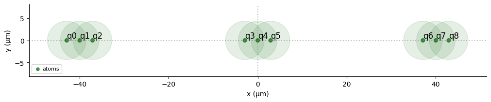
We first consider clusters of \(1, 2\) and \(3\) atoms under resonant (\(\delta = 0\)) driving. If all the atoms are placed within each other’s blockade volume, only one excitation per group will be possible at a time. The Rabi frequency will be enhanced by \(\sqrt{N}\)
[2]:
def occupation(reg, j):
    r = qutip.basis(2, 0)
    N = len(reg.qubits)
    prod = [qutip.qeye(2) for _ in range(N)]
    prod[j] = r * r.dag()
    return qutip.tensor(prod)
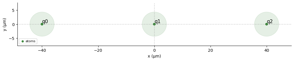
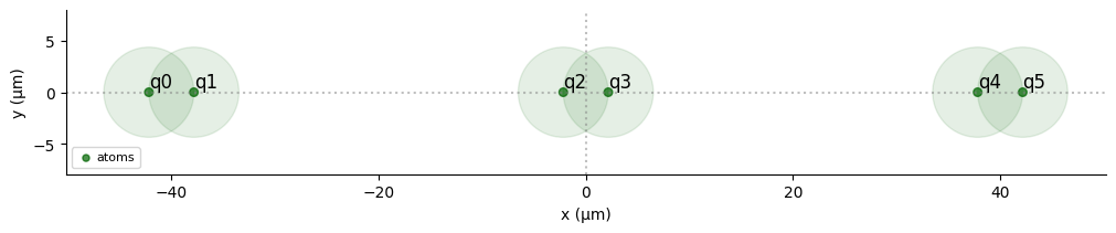
Given a value of the maximum Rabi Frequency applied to the atoms, we can calculate the corresponding blockade radius using the rydberg_blockade_radius() method from MockDevice. We use this to arrange clusters of atoms which will experience this blockade effect:
[3]:
Omega_max = 2 * 2 * np.pi
R_blockade = MockDevice.rydberg_blockade_radius(Omega_max)
print(f"Blockade Radius is: {R_blockade}µm.")
groups = 3


def blockade_cluster(N):
    atom_coords = [
        ((R_blockade / N) * x + 40 * group, 0)
        for group in range(groups)
        for x in range(1, N + 1)
    ]
    reg = Register.from_coordinates(atom_coords, prefix="q")
    reg.draw(
        blockade_radius=R_blockade, draw_half_radius=True, draw_graph=False
    )

    resonant_pulse = Pulse.ConstantPulse(1500, Omega_max, 0.0, 0.0)

    seq = Sequence(reg, MockDevice)
    seq.declare_channel("ising", "rydberg_global")
    seq.add(resonant_pulse, "ising")

    simul = QutipEmulator.from_sequence(seq, sampling_rate=0.2)

    obs = [
        sum(occupation(reg, j) for j in range(i, i + N))
        for i in range(0, groups * N, N)
    ]

    res = simul.run(progress_bar=True, method="bdf")
    return res.expect(obs)
Blockade Radius is: 8.692279598222772µm.
Next we run blockade_cluster(N), which runs the simulation, for clusters of sizes \(N \in \{1,2,3\}\):
[4]:
data = [blockade_cluster(N) for N in [1, 2, 3]]
10.0%. Run time:   0.01s. Est. time left: 00:00:00:00
20.0%. Run time:   0.02s. Est. time left: 00:00:00:00
30.0%. Run time:   0.02s. Est. time left: 00:00:00:00
40.0%. Run time:   0.03s. Est. time left: 00:00:00:00
50.0%. Run time:   0.04s. Est. time left: 00:00:00:00
60.0%. Run time:   0.05s. Est. time left: 00:00:00:00
70.0%. Run time:   0.07s. Est. time left: 00:00:00:00
80.0%. Run time:   0.07s. Est. time left: 00:00:00:00
90.0%. Run time:   0.08s. Est. time left: 00:00:00:00
Total run time:   0.08s
10.0%. Run time:   0.02s. Est. time left: 00:00:00:00
20.0%. Run time:   0.05s. Est. time left: 00:00:00:00
30.0%. Run time:   0.07s. Est. time left: 00:00:00:00
40.0%. Run time:   0.13s. Est. time left: 00:00:00:00
50.0%. Run time:   0.17s. Est. time left: 00:00:00:00
60.0%. Run time:   0.22s. Est. time left: 00:00:00:00
70.0%. Run time:   0.27s. Est. time left: 00:00:00:00
80.0%. Run time:   0.34s. Est. time left: 00:00:00:00
90.0%. Run time:   0.39s. Est. time left: 00:00:00:00
Total run time:   0.45s
10.0%. Run time:   1.02s. Est. time left: 00:00:00:09
20.0%. Run time:   1.92s. Est. time left: 00:00:00:07
30.0%. Run time:   2.74s. Est. time left: 00:00:00:06
40.0%. Run time:   3.70s. Est. time left: 00:00:00:05
50.0%. Run time:   4.74s. Est. time left: 00:00:00:04
60.0%. Run time:   5.74s. Est. time left: 00:00:00:03
70.0%. Run time:   7.16s. Est. time left: 00:00:00:03
80.0%. Run time:   8.58s. Est. time left: 00:00:00:02
90.0%. Run time:  10.25s. Est. time left: 00:00:00:01
Total run time:  12.29s
We now plot the probability that a Rydberg state withing the cluster is occupied (by summing the expectation values of the \(|r\rangle\langle r|_i\) operators for each cluster) as it evolves in time, revealing the Rabi frequency of each configuration:
[5]:
fig, ax = plt.subplots(1, 3, figsize=(18, 3))
for N, expectation in enumerate(data):
    ax[N].set_xlabel(r"Time ($µs$)", fontsize=10)
    ax[N].set_ylabel(r"Probability of $|r\rangle$", fontsize=10)
    ax[N].set_title(f"Atoms per cluster N = {N+1}", fontsize=12)
    avg = sum(expectation) / groups
    ax[N].plot(np.arange(len(avg)) / 1000, avg)
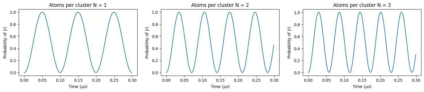
Only one excitation will be shared between the atoms on each cluster. Notice how the Rabi frequency increases by a factor of \(\sqrt{N}\)
2. Ordered Crystalline phases
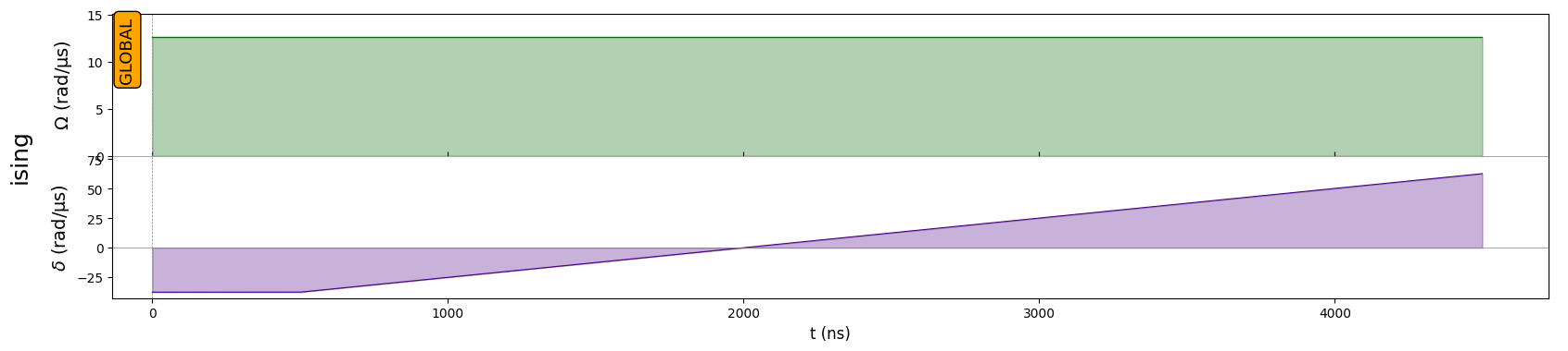
The pulse sequence that we will prepare is based on the following parameters:
[6]:
# Parameters in rad/µs and ns
delta_0 = -6 * 2 * np.pi
delta_f = 10 * 2 * np.pi
Omega_max = 2 * 2 * np.pi
t_rise = 500
t_stop = 4500
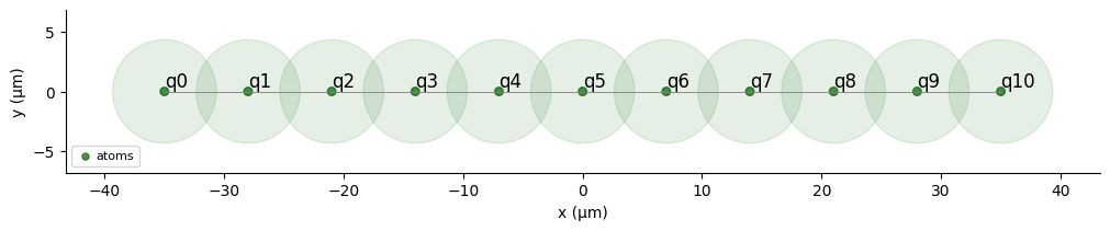
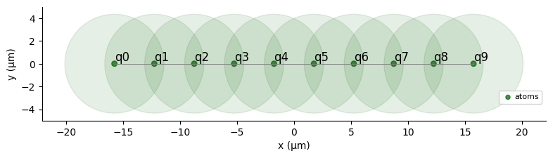
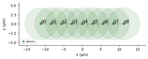
We calculate the blockade radius from the maximal applied Rabi frequency:
[7]:
R_blockade = MockDevice.rydberg_blockade_radius(Omega_max)
a = 7.0

reg = Register.rectangle(1, 11, spacing=a, prefix="q")
print(f"Blockade Radius is: {R_blockade}µm.")
reg.draw(blockade_radius=R_blockade, draw_half_radius=True)
Blockade Radius is: 8.692279598222772µm.
Create the pulses using Pulser objects:
[8]:
hold = ConstantWaveform(t_rise, delta_0)
excite = RampWaveform(t_stop - t_rise, delta_0, delta_f)
sweep = Pulse.ConstantAmplitude(
    Omega_max, CompositeWaveform(hold, excite), 0.0
)
[9]:
seq = Sequence(reg, MockDevice)
seq.declare_channel("ising", "rydberg_global")

seq.add(sweep, "ising")

seq.draw()
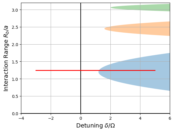
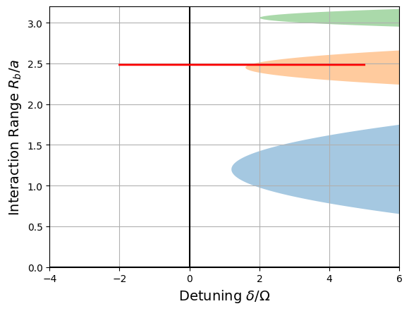
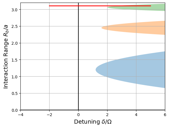
The pulse sequence we just created corresponds a path in the Phase space of the ground state, which we represent schematically with the following function:
[10]:
def phase_diagram(seq):
    ratio = []
    for x in seq._schedule["ising"]:
        if isinstance(x.type, Pulse):
            ratio += list(x.type.detuning.samples / Omega_max)

    fig, ax = plt.subplots()
    ax.grid(True, which="both")

    ax.set_ylabel(r"Interaction Range $R_b/a$", fontsize=14)
    ax.set_xlabel(r"Detuning $\delta/\Omega$", fontsize=14)
    ax.set_xlim(-4, 6)
    ax.set_ylim(0, 3.2)
    ax.axhline(y=0, color="k")
    ax.axvline(x=0, color="k")

    y = np.arange(0.0, 5, 0.01)
    x = 2 * (0.6 + 8 * (y - 1.2) ** 2)
    ax.fill_between(x, y, alpha=0.4)

    y = np.arange(0.0, 5, 0.01)
    x = 2 * (0.8 + 50 * (y - 2.45) ** 2)
    ax.fill_between(x, y, alpha=0.4)

    y = np.arange(0.0, 5, 0.01)
    x = 2 * (1.0 + 170 * (y - 3.06) ** 2)
    ax.fill_between(x, y, alpha=0.4)

    ax.plot(np.array(ratio), np.full(len(ratio), R_blockade / a), "red", lw=2)
    plt.show()
[11]:
phase_diagram(seq)
2.1 Simulation
We run our simulation, for a list of observables corresponding to \(|r\rangle \langle r|_j\) for each atom in the register:
[12]:
simul = QutipEmulator.from_sequence(seq, sampling_rate=0.1)

occup_list = [occupation(reg, j) for j in range(len(reg.qubits))]

res = simul.run(progress_bar=True)
occupations = res.expect(occup_list)
10.0%. Run time:   0.76s. Est. time left: 00:00:00:06
20.0%. Run time:   1.61s. Est. time left: 00:00:00:06
30.0%. Run time:   2.55s. Est. time left: 00:00:00:05
40.0%. Run time:   3.27s. Est. time left: 00:00:00:04
50.0%. Run time:   3.86s. Est. time left: 00:00:00:03
60.0%. Run time:   4.40s. Est. time left: 00:00:00:02
70.0%. Run time:   4.99s. Est. time left: 00:00:00:02
80.0%. Run time:   5.60s. Est. time left: 00:00:00:01
90.0%. Run time:   6.35s. Est. time left: 00:00:00:00
Total run time:   7.21s
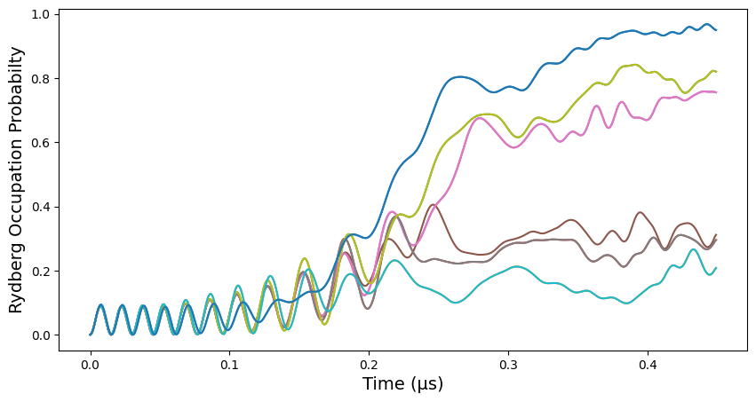
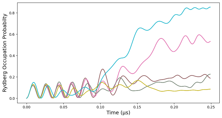
The following function plots the evolution of the expectation values with respect to time:
[13]:
def plot_evolution(results):
    plt.figure(figsize=(10, 5))
    plt.xlabel("Time (µs)", fontsize=14)
    plt.ylabel("Rydberg Occupation Probabilty", fontsize=14)
    for expv in results:
        plt.plot(np.arange(len(expv)) / 1000, expv)

    plt.show()
[14]:
plot_evolution(occupations)
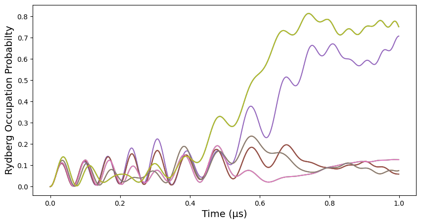
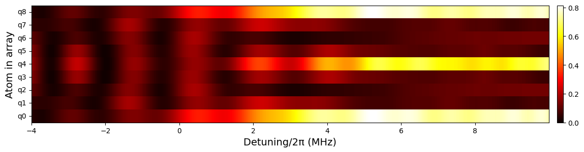
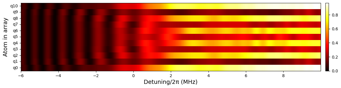
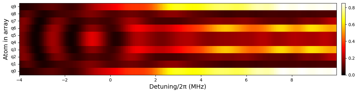
We finally plot the probability of occupation of the Rydberg level with respect to the values of detuning, for each atom in the array:
[15]:
def heat_detuning(data, start, end):
    N = len(reg.qubits)
    time_window = []
    x = []
    detunings = simul.samples_obj.to_nested_dict()["Global"]["ground-rydberg"][
        "det"
    ][[int(1000 * t) for t in simul.evaluation_times[:-1]]]

    for t, d in enumerate(detunings):
        if start <= d <= end:
            time_window.append(t)
            x.append(d / (2 * np.pi))

    y = np.arange(1, N + 1)

    X, Y = np.meshgrid(x, y)
    Z = np.array(data)[:, time_window]

    plt.figure(figsize=(14, 3))
    plt.pcolormesh(X, Y, Z, cmap="hot", shading="auto")
    plt.xlabel("Detuning/2π (MHz)", fontsize=14)
    plt.ylabel("Atom in array", fontsize=14)
    plt.yticks(range(1, N + 1), [f"q{i}" for i in range(N)], va="center")
    plt.colorbar(fraction=0.047, pad=0.015)

    plt.show()
[16]:
heat_detuning(occupations, delta_0, delta_f)
2.2 Rydberg Crystals: \(Z_3\) Order
To arrive at a different phase, we reduce the interatomic distance \(a\), thus increasing the interaction range between the atoms. This will lead to a \(Z_3\) ordered phase:
[17]:
a = 3.5
reg = Register.rectangle(1, 10, spacing=a, prefix="q")

delta_0 = -4 * 2 * np.pi
delta_f = 10 * 2 * np.pi
Omega_max = 2.0 * 2 * np.pi  # btw 1.8-2 * 2pi MHz
t_rise = 600
t_stop = 2500
R_blockade = MockDevice.rydberg_blockade_radius(Omega_max)
reg.draw(blockade_radius=R_blockade, draw_half_radius=True)

#
hold = ConstantWaveform(t_rise, delta_0)
excite = RampWaveform(t_stop - t_rise, delta_0, delta_f)
sweep = Pulse.ConstantAmplitude(
    Omega_max, CompositeWaveform(hold, excite), 0.0
)
#
seq = Sequence(reg, MockDevice)
seq.declare_channel("ising", "rydberg_global")
seq.add(sweep, "ising")

phase_diagram(seq)

simul = QutipEmulator.from_sequence(seq, sampling_rate=0.1)

occup_list = [occupation(reg, j) for j in range(len(reg.qubits))]

res = simul.run(progress_bar=True, method="bdf")

occupations = res.expect(occup_list)

plot_evolution(occupations)
heat_detuning(occupations, delta_0, delta_f)
10.0%. Run time:   2.20s. Est. time left: 00:00:00:19
20.0%. Run time:   4.31s. Est. time left: 00:00:00:17
30.0%. Run time:   6.38s. Est. time left: 00:00:00:14
40.0%. Run time:   8.46s. Est. time left: 00:00:00:12
50.0%. Run time:  10.56s. Est. time left: 00:00:00:10
60.0%. Run time:  12.80s. Est. time left: 00:00:00:08
70.0%. Run time:  14.89s. Est. time left: 00:00:00:06
80.0%. Run time:  16.99s. Est. time left: 00:00:00:04
90.0%. Run time:  19.08s. Est. time left: 00:00:00:02
Total run time:  21.14s
2.3 Rydberg Crystals: \(Z_4\) Order
Decreasing even more the interatomic distance leads to a \(Z_4\) order. The magnitude of the Rydberg interaction with respect to that of the applied pulses means our solver has to control terms with a wider range, thus leading to longer simulation times:
[18]:
a = 2.8
reg = Register.rectangle(1, 9, spacing=a, prefix="q")

# Parameters in rad/µs and ns

delta_0 = -4 * 2 * np.pi
delta_f = 10 * 2 * np.pi
Omega_max = 2.0 * 2 * np.pi  # btw 1.8-2 2pi*MHz
t_rise = 600
t_stop = 2500
R_blockade = MockDevice.rydberg_blockade_radius(Omega_max)
reg.draw(blockade_radius=R_blockade, draw_half_radius=True)

#
hold = ConstantWaveform(t_rise, delta_0)
excite = RampWaveform(t_stop - t_rise, delta_0, delta_f)
sweep = Pulse.ConstantAmplitude(
    Omega_max, CompositeWaveform(hold, excite), 0.0
)

#
seq = Sequence(reg, MockDevice)
seq.declare_channel("ising", "rydberg_global")
seq.add(sweep, "ising")

phase_diagram(seq)

simul = QutipEmulator.from_sequence(seq, sampling_rate=0.4)

occup_list = [occupation(reg, j) for j in range(len(reg.qubits))]

#
res = simul.run(progress_bar=True, method="bdf")
occupations = res.expect(occup_list)

plot_evolution(occupations)
heat_detuning(occupations, delta_0, delta_f)
10.0%. Run time:   4.70s. Est. time left: 00:00:00:42
20.0%. Run time:  10.75s. Est. time left: 00:00:00:42
30.0%. Run time:  16.96s. Est. time left: 00:00:00:39
40.0%. Run time:  24.73s. Est. time left: 00:00:00:37
50.0%. Run time:  32.96s. Est. time left: 00:00:00:32
60.0%. Run time:  39.45s. Est. time left: 00:00:00:26
70.0%. Run time:  44.43s. Est. time left: 00:00:00:19
80.0%. Run time:  49.02s. Est. time left: 00:00:00:12
90.0%. Run time:  53.25s. Est. time left: 00:00:00:05
Total run time:  58.02s