Execution on an Emulator

What you will learn:

• what a Backend is for;

• what types of emulator Backend exist;

• how to choose the best Backend for your needs;

• how to execute a Sequence on an emulator Backend and retrieve the results.

Introduction

When the time comes to execute a Pulser sequence, there are many options: one can choose to execute it on a QPU or on an emulator, which might happen locally or remotely. All these options are accessible through an unified interface we call a Backend.

This tutorial is a step-by-step guide on how to use emulator backends for Pulser sequence execution.

Although the final goal of a quantum algorithm is to run on a QPU, we always recommend starting on an emulator. Emulators are more readily available, and at lower cost, in addition to providing much more information than a QPU, which can only measure bitstrings. When running on an emulator we recommend first doing some exploratory runs locally to ensure you’re doing the right thing, before submitting your heavier jobs to be run on the cluster through the cloud.

Info

Go to this tutorial for more information on how to execute a Pulser sequence on a QPU backend.

1. Creating the Pulse Sequence

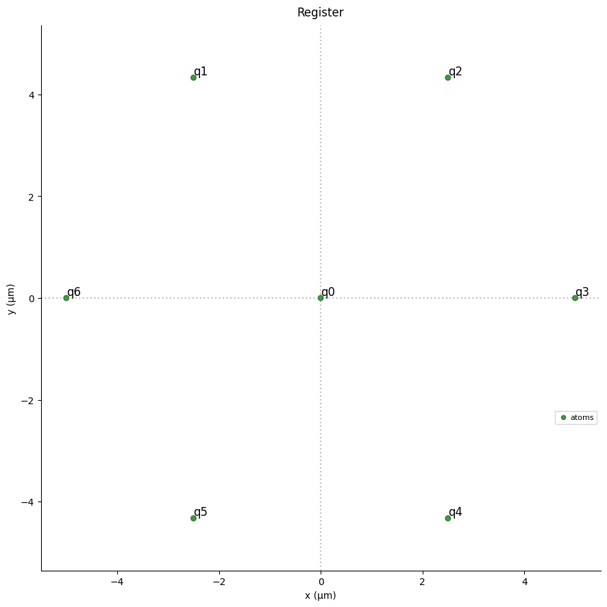
The first step is to create the sequence that we want to execute. Let’s prepare an AFM state (as in the introduction tutorial), but this time on a hexagon of 7 atoms and using another set of pulses. Since it will be executed on an emulator, we don’t have any constraint on the Device or the Register used, so the Device could be a VirtualDevice like a MockDevice.

import numpy as np
import pulser
import pulser_simulation

# 1. Picking a Device
device = pulser.AnalogDevice

# 2. Creating the Register
R_interatomic = 5  # um
register = pulser.Register.hexagon(1, R_interatomic, prefix="q")

seq = pulser.Sequence(register, device)

# 3. Picking the channels
seq.declare_channel("rydberg_global", "rydberg_global")

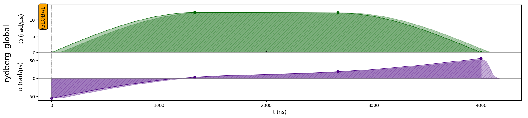
# 4. Adding the pulses

# Parameters in rad/µs
U = device.interaction_coeff / R_interatomic**6

# Time parameters
total_duration = 4000  # in ns
interp_pts = np.linspace(0, 1, 4)  # between 0 and 1

seq.add(
    pulser.Pulse(
        pulser.InterpolatedWaveform(
            total_duration,
            U * np.array([1e-9, 0.22, 0.2181, 1e-9]),
            times=interp_pts,
        ),
        pulser.InterpolatedWaveform(
            total_duration,
            U * np.array([-1, 0.0556, 0.332, 1]),
            times=interp_pts,
        ),
        0,
    ),
    "rydberg_global",
)

seq.draw(draw_register=True)

2. Running on a local backend

It is now time to select and initialize the backend. We will start running things locally using the QutipBackendV2 (from pulser_simulation). It uses qutip to emulate the sequence execution locally.

Keep in mind that other emulators are available, and the full list is available here.

Tip

You can acess all backends that are available on your system via the pulser.backends module so you don’t need to explicitly import them.

Upon creation, all backends require the sequence they will execute.

qutip_bknd = pulser.backends.QutipBackendV2(seq)
qutip_results = qutip_bknd.run()

Emulating Trajectory 1/1

As defined in their default configurations, all backends return the bitstrings at the final time, and QutipBackendV2 also returns the final state. You can check the default configuration of any emulator backend by printing its default_config:

print(pulser.backends.QutipBackendV2.default_config)

QutipConfig(
    callbacks=(),
    observables=(bitstrings:fee775fe-37ca-491e-a9fd-81fa0a67324c, state:6add9958-e748-4486-94c2-00f48e8d3c12),
    default_evaluation_times=array([1.]),
    initial_state=None,
    with_modulation=False,
    interaction_matrix=None,
    prefer_device_noise_model=False,
    noise_model=NoiseModel(noise_types=()),
    n_trajectories=1,
    sampling_rate=1.0,
    solver=<Solver.DEFAULT: 'default'>,
    progress_bar=False,
    default_num_shots=1000,
)

• For the detailed explanation of each parameter, please consult the API reference.

• Check out this section for more details and best practices on how to configure an emulation.

3. Retrieving the Results

Info

For more details on how to extract values from Results, consult this page.

For any Results returned from an EmulatorBackend, we can query the contents of a result by printing them. As we can see below, QutipBackendV2 returns the bitstrings and quantum state at the final time by default.

Note

The times at which a result is measured are presented as a fraction of the sequence duration, so a time of 1.0 always represent the final time.

print(qutip_results)

Results
-------
Stored results: ['bitstrings', 'state']
Evaluation times per result: {'bitstrings': [1.0], 'state': [1.0]}
Atom order in states and bitstrings: ('q0', 'q1', 'q2', 'q3', 'q4', 'q5', 'q6')
Total sequence duration: 4000 ns

We can query the bitstrings at the final time, if present, using a dedicated property.

print(qutip_results.final_bitstrings)

Counter({'0101010': 514, '0010101': 486})

The same is true for the final state, which we combine below with a special method of QutipState to converts it to a qutip.Qobj.

qutip_state = qutip_results.final_state
# This is particular to `QutipState`
qutip_state.to_qobj()

Quantum object: dims=[[2, 2, 2, 2, 2, 2, 2], [1]], shape=(128, 1), type='ket', dtype=Dense$$\left(\begin{array}{cc}-1.753\times10^{ -4 }\\-4.517\times10^{ -8 }\\-4.517\times10^{ -8 }\\-1.274\times10^{ -8 }\\-4.517\times10^{ -8 }\\\vdots\\-0.001\\3.746\times10^{ -4 }\\-0.001\\-0.001\\-6.008\times10^{ -6 }\end{array}\right)$$

For each stored result, the attribute having its name provides the list of result of that type obtained at each of its evaluation times.

We can also use this to access the bitstrings measured at the final time.

Note

• You can get a list of all the stored results with get_result_tags().

• For each of these stored results, you can get the list of evaluation times with get_result_times().

print("Stored results' tags:", qutip_results.get_result_tags())
print(
    "Evaluation times for 'bitstrings':",
    qutip_results.get_result_times("bitstrings"),
)
# These are equivalent
qutip_results.get_result("bitstrings", 1.0)
qutip_results.bitstrings[-1]

Stored results' tags: ['bitstrings', 'state']
Evaluation times for 'bitstrings': [1.0]

Counter({'0101010': 514, '0010101': 486})

4. Configuring the Emulation

Info

For more details on how to configure an emulation with Observables, consult this page.

The contents of the result (i.e. the quantities it stores at specific evaluation times) depend on the Observables defined in the EmulationConfig of an emulator backend. Each Emulator backends has a configuration given as an instance of the EmulationConfig class.

• As can be seen from the docs, this class defines a few generally applicable configuration options, and then accepts backend specific options as keyword arguments.

• Each backend defines its favoured EmulationConfig subclass via EmulatorBackend.config_type (such as QutipConfig for QutipBackendV2) that makes explicit the specific options for that backend. You can find a generic code to define a configuration from EmulatorBackend.config_type here.

• In the absence of a custom config argument, the emulator will use EmulatorConfig.default_config.

To showcase the flexibility of emulation backends specifically, we will configure QutipBackendV2 to return the overlap with the Anti-Ferromagnetic state \(\frac{1}{\sqrt{2}} \left(\left|grgrgrg\right>+\left|ggrgrgr\right>\right)\) halfway through the sequence and at the end, which can be done using the Fidelity observable documented here.

Tip

• Fidelity is an example of a State-dependent observable. Take a look at this section for more details on how to handle this type of observable.

• A Fidelity observable is normally added to the Results as fidelity, but in order to make it more specific, we use tag_suffix to make it present itself as fidelity_AFM_7. This option is present for all observables, but it mostly makes sense for observable types that could show up multiple times with different parameters.

• Rather than defining an EmulationConfig from scratch, the example below starts from the backend’s default_config and uses EmulationConfig.with_changes() to add the fidelity observable.

# Pick a backend, here we chose QutipBackendV2
emu_backend_class = pulser_simulation.QutipBackendV2

config_class = emu_backend_class.config_type  # In this case, `QutipConfig`
state_class = config_class.state_type  # In this case, `QutipState`

fidelity_state = state_class.from_state_amplitudes(
    eigenstates=("r", "g"),
    amplitudes={"grgrgrg": 1 / np.sqrt(2), "ggrgrgr": 1 / np.sqrt(2)},
)
fidelity = pulser.backend.Fidelity(
    state=fidelity_state, tag_suffix="AFM_7", evaluation_times=[0.5, 1.0]
)

# Start from the default_config and add the Fidelity observable
default_config = emu_backend_class.default_config
new_observables = list(default_config.observables) + [fidelity]
config = default_config.with_changes(observables=new_observables)
print(config)

QutipConfig(
    callbacks=(),
    observables=(bitstrings:fee775fe-37ca-491e-a9fd-81fa0a67324c, state:6add9958-e748-4486-94c2-00f48e8d3c12, fidelity_AFM_7:d093b4fc-8183-401d-9611-37076313cc4a),
    default_evaluation_times=array([1.]),
    initial_state=None,
    with_modulation=False,
    interaction_matrix=None,
    prefer_device_noise_model=False,
    noise_model=NoiseModel(noise_types=()),
    n_trajectories=1,
    sampling_rate=1.0,
    solver=<Solver.DEFAULT: 'default'>,
    progress_bar=False,
    default_num_shots=1000,
)

Now that we have defined a custom config, we can create a new backend, run the emulation, and analyze the results.

qutip_bknd_custom = emu_backend_class(seq, config=config)
custom_results = qutip_bknd_custom.run()
print(custom_results)

Emulating Trajectory 1/1
Results
-------
Stored results: ['fidelity_AFM_7', 'bitstrings', 'state']
Evaluation times per result: {'fidelity_AFM_7': [0.5, 1.0], 'bitstrings': [1.0], 'state': [1.0]}
Atom order in states and bitstrings: ('q0', 'q1', 'q2', 'q3', 'q4', 'q5', 'q6')
Total sequence duration: 4000 ns

Since we requested the fidelity at two different times, asking for the result times will reflect this.

print(custom_results.get_result_times("fidelity_AFM_7"))

[0.5, 1.0]

The two fidelities are in the results in chronological order.

print(custom_results.fidelity_AFM_7[0])
print(custom_results.fidelity_AFM_7[1])

0.2415769618200006
0.9998684338132205

5. Running Remotely

Now that we understand the behaviour of our sequence, and how to use emulator backends locally, let’s run the sequence on a pair of remote backends

• EmuFreeBackendV2 (from pulser_pasqal): Executes the sequence on QutipBackendV2 remotely in the cloud.

• EmuMPSBackend (from pulser_pasqal): Executes the sequence on MPSBackend remotely in the cloud.

Info

A full list of available backends is available in the backends module API reference.

Notice that running things remotely requires us to provide a RemoteConnection object. To execute a Sequence on Pasqal cloud, the appropriate connection object is:

from pulser_pasqal import PasqalCloud

connection = PasqalCloud(
    username=USERNAME,  # Your username or email address for the Pasqal Cloud Platform
    project_id=PROJECT_ID,  # The ID of the project associated to your account
    password=PASSWORD,  # The password for your Pasqal Cloud Platform account
)

We now have a connection to the cloud. However, before creating the backends, let us create a custom EmulationConfig with a Fidelity observable again; only this time around, we’ll define the state using the agnostic StateRepr type, which is appropriate for all remote backends.

Tip

When passing a State or Operator to an observable for remote use, or when passing the initial_state to EmulationConfig, it is recommended to use the StateRepr and OperatorRepr classes, which will work for all remote backends but not necessarily for local ones.

Warning

When running remotely, the configuration and emulation results have to be serialized. Since quantum states are potentially extremely large, the StateResult observable is disabled, and State and Operator classes will only serialize if they were created from an abstract representation.

remote_fidelity_state = pulser.backend.StateRepr.from_state_amplitudes(
    eigenstates=("r", "g"),
    amplitudes={"grgrgrg": 1 / np.sqrt(2), "ggrgrgr": 1 / np.sqrt(2)},
)
remote_fidelity = pulser.backend.Fidelity(
    state=remote_fidelity_state,
    tag_suffix="AFM_7",
    evaluation_times=[0.5, 1.0],
)

remote_config = pulser.backend.EmulationConfig(
    observables=[remote_fidelity],
)

Now that we have a proper Sequence, EmulationConfig and Connection, we can create the EmuFreeBackendV2 and EmuMPSBackend with which we want to run the emulation.

free_bknd = pulser.backends.EmuFreeBackendV2(
    seq, config=remote_config, connection=connection
)
mps_bknd = pulser.backends.EmuMPSBackend(
    seq, config=remote_config, connection=connection
)

Warning

Remote backends support the submission of multiple jobs on the same run() call, so the returned RemoteResults instance is a sequence of Results. This feature is most useful when combined with a parametrized sequence for execution on a QPU backend.

By default, a call to run() will submit a single job so the resulting RemoteResults will contain a single Results instance.

free_results = free_bknd.run()
print(f"Submitted batch {free_results.batch_id} to EmuFreeBackendV2")
mps_results = mps_bknd.run()
print(f"Submitted batch {mps_results.batch_id} to EmuMPSBackend")

Submitted batch 05fe761e-9a5f-468d-8de0-a2629808d5e1 to EmuFreeBackendV2
Submitted batch ef97bbf1-3450-4fbb-a386-969d759221a2 to EmuMPSBackend

Tip

You can restore the RemoteResults object associated to a batch at anytime from its batch ID (see results.batch_id above) by running

pulser.backendRemoteResults(batch_id, connection)

For remote backends, the object returned is a RemoteResults instance, which uses the connection to fetch the results once they are ready. To check the status of the batch, we can run:

print(free_results.get_batch_status())
print(mps_results.get_batch_status())

BatchStatus.DONE
BatchStatus.DONE

When the batch states shows as DONE, the results can be accessed. We can use get_available_results to see the results as they become available.

print("Got results:", free_results.get_available_results(), "\n")
print(free_results[-1])

print("\nFidelities:", free_results[-1].fidelity_AFM_7)

Got results: {'ac79ec19-154a-491b-a467-3c105d9f73c8': <pulser.backend.results.Results object at 0x7d8a5830a540>}

Results
-------
Stored results: ['fidelity_AFM_7']
Evaluation times per result: {'fidelity_AFM_7': [0.5, 1.0]}
Atom order in states and bitstrings: ('q0', 'q1', 'q2', 'q3', 'q4', 'q5', 'q6')
Total sequence duration: 4000 ns

Fidelities: [0.2415769618200006, 0.9998684338132205]

In addition to the above, MPSBackend, SVBackend and their derivatives, such as the remote EmuMPSBackend store runtime statistics in the Results. For more information about this, please see the corresponding documentation.

print(mps_results[-1])
print("\nFidelities:", mps_results[-1].fidelity_AFM_7)

Results
-------
Stored results: ['statistics', 'fidelity_AFM_7']
Evaluation times per result: {'statistics': [0.0025, 0.005, 0.0075, 0.01, 0.0125, 0.015, 0.0175, 0.02, 0.0225, 0.025, 0.0275, 0.03, 0.0325, 0.035, 0.0375, 0.04, 0.0425, 0.045, 0.0475, 0.05, 0.0525, 0.055, 0.0575, 0.06, 0.0625, 0.065, 0.0675, 0.07, 0.0725, 0.075, 0.0775, 0.08, 0.0825, 0.085, 0.0875, 0.09, 0.0925, 0.095, 0.0975, 0.1, 0.1025, 0.105, 0.1075, 0.11, 0.1125, 0.115, 0.1175, 0.12, 0.1225, 0.125, 0.1275, 0.13, 0.1325, 0.135, 0.1375, 0.14, 0.1425, 0.145, 0.1475, 0.15, 0.1525, 0.155, 0.1575, 0.16, 0.1625, 0.165, 0.1675, 0.17, 0.1725, 0.175, 0.1775, 0.18, 0.1825, 0.185, 0.1875, 0.19, 0.1925, 0.195, 0.1975, 0.2, 0.2025, 0.205, 0.2075, 0.21, 0.2125, 0.215, 0.2175, 0.22, 0.2225, 0.225, 0.2275, 0.23, 0.2325, 0.235, 0.2375, 0.24, 0.2425, 0.245, 0.2475, 0.25, 0.2525, 0.255, 0.2575, 0.26, 0.2625, 0.265, 0.2675, 0.27, 0.2725, 0.275, 0.2775, 0.28, 0.2825, 0.285, 0.2875, 0.29, 0.2925, 0.295, 0.2975, 0.3, 0.3025, 0.305, 0.3075, 0.31, 0.3125, 0.315, 0.3175, 0.32, 0.3225, 0.325, 0.3275, 0.33, 0.3325, 0.335, 0.3375, 0.34, 0.3425, 0.345, 0.3475, 0.35, 0.3525, 0.355, 0.3575, 0.36, 0.3625, 0.365, 0.3675, 0.37, 0.3725, 0.375, 0.3775, 0.38, 0.3825, 0.385, 0.3875, 0.39, 0.3925, 0.395, 0.3975, 0.4, 0.4025, 0.405, 0.4075, 0.41, 0.4125, 0.415, 0.4175, 0.42, 0.4225, 0.425, 0.4275, 0.43, 0.4325, 0.435, 0.4375, 0.44, 0.4425, 0.445, 0.4475, 0.45, 0.4525, 0.455, 0.4575, 0.46, 0.4625, 0.465, 0.4675, 0.47, 0.4725, 0.475, 0.4775, 0.48, 0.4825, 0.485, 0.4875, 0.49, 0.4925, 0.495, 0.4975, 0.5, 0.5025, 0.505, 0.5075, 0.51, 0.5125, 0.515, 0.5175, 0.52, 0.5225, 0.525, 0.5275, 0.53, 0.5325, 0.535, 0.5375, 0.54, 0.5425, 0.545, 0.5475, 0.55, 0.5525, 0.555, 0.5575, 0.56, 0.5625, 0.565, 0.5675, 0.57, 0.5725, 0.575, 0.5775, 0.58, 0.5825, 0.585, 0.5875, 0.59, 0.5925, 0.595, 0.5975, 0.6, 0.6025, 0.605, 0.6075, 0.61, 0.6125, 0.615, 0.6175, 0.62, 0.6225, 0.625, 0.6275, 0.63, 0.6325, 0.635, 0.6375, 0.64, 0.6425, 0.645, 0.6475, 0.65, 0.6525, 0.655, 0.6575, 0.66, 0.6625, 0.665, 0.6675, 0.67, 0.6725, 0.675, 0.6775, 0.68, 0.6825, 0.685, 0.6875, 0.69, 0.6925, 0.695, 0.6975, 0.7, 0.7025, 0.705, 0.7075, 0.71, 0.7125, 0.715, 0.7175, 0.72, 0.7225, 0.725, 0.7275, 0.73, 0.7325, 0.735, 0.7375, 0.74, 0.7425, 0.745, 0.7475, 0.75, 0.7525, 0.755, 0.7575, 0.76, 0.7625, 0.765, 0.7675, 0.77, 0.7725, 0.775, 0.7775, 0.78, 0.7825, 0.785, 0.7875, 0.79, 0.7925, 0.795, 0.7975, 0.8, 0.8025, 0.805, 0.8075, 0.81, 0.8125, 0.815, 0.8175, 0.82, 0.8225, 0.825, 0.8275, 0.83, 0.8325, 0.835, 0.8375, 0.84, 0.8425, 0.845, 0.8475, 0.85, 0.8525, 0.855, 0.8575, 0.86, 0.8625, 0.865, 0.8675, 0.87, 0.8725, 0.875, 0.8775, 0.88, 0.8825, 0.885, 0.8875, 0.89, 0.8925, 0.895, 0.8975, 0.9, 0.9025, 0.905, 0.9075, 0.91, 0.9125, 0.915, 0.9175, 0.92, 0.9225, 0.925, 0.9275, 0.93, 0.9325, 0.935, 0.9375, 0.94, 0.9425, 0.945, 0.9475, 0.95, 0.9525, 0.955, 0.9575, 0.96, 0.9625, 0.965, 0.9675, 0.97, 0.9725, 0.975, 0.9775, 0.98, 0.9825, 0.985, 0.9875, 0.99, 0.9925, 0.995, 0.9975, 1.0], 'fidelity_AFM_7': [0.5, 1.0]}
Atom order in states and bitstrings: ('q0', 'q1', 'q2', 'q3', 'q4', 'q5', 'q6')
Total sequence duration: 4000 ns

Fidelities: [0.24161613994468908, 0.999885389768192]

6. Alternative user interfaces for using remote backends

Once you have created a Pulser sequence, you can also use specialized Python SDKs to send it for execution:

• the pasqal-cloud Python SDK, developed by PASQAL and used under-the-hood by Pulser’s remote backends.

• Azure’s Quantum Development Kit (QDK) which you can use by creating an Azure Quantum workspace directly integrated with PASQAL emulators and QPU.