Pulse Sequence Creation

import numpy as np
import pulser
from pprint import pprint

1. Creating the Register

The Register defines the positions of the atoms and their names of each one. There are multiple ways of defining a Register, the most customizable one being to create a dictionary that associates a name (the key) to a cooordinate (the value).

L = 4
square = np.array([[i, j] for i in range(L) for j in range(L)], dtype=float)
square -= np.mean(square, axis=0)
square *= 5

qubits = dict(enumerate(square))
reg = pulser.Register(qubits)

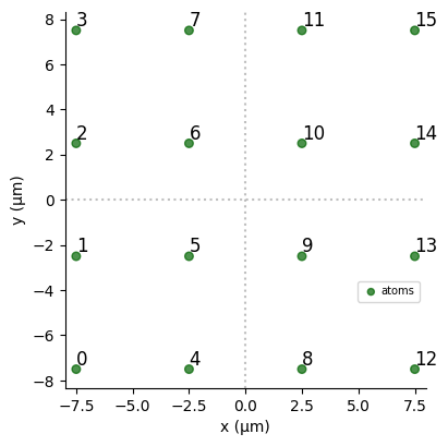
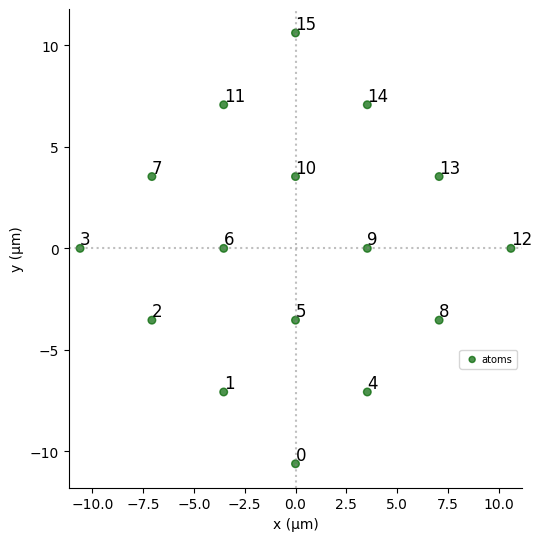
The Register class provides some useful features, like the ability to visualise the array and to make a rotated copy.

print("The original array:")
reg.draw()
reg1 = reg.rotated(45)  # Rotate by 45 degrees
print("The rotated array:")
reg1.draw()

The original array:

The rotated array:

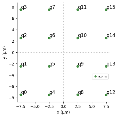
If one doesn’t particularly care about the name given to the qubits, one can also create a Register just from a list of coordinates (using the Register.from_coordinates class method). In this case, the qubit ID’s are just numbered, starting from 0, in the order they are provided in, with the option of adding a common prefix before each number. Also, it automatically centers the entire array around the origin, an option that can be disabled if desired.

reg2 = pulser.Register.from_coordinates(
    square, prefix="q"
)  # All qubit IDs will start with 'q'
reg2.draw()

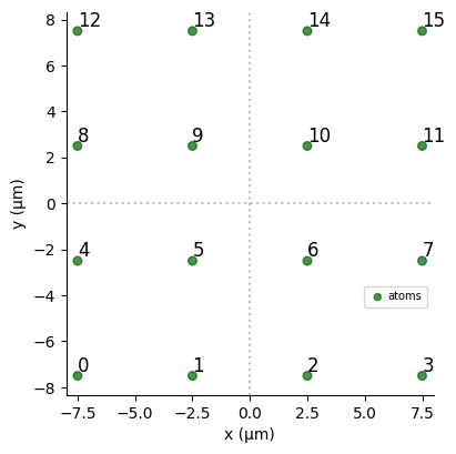
Furthermore, there are also built-in class methods from creation of common array patterns, namely: - Square lattices in rectangular or square shapes - Triangular lattices

We could, thus, create the same square array as before by doing:

reg3 = pulser.Register.square(4, spacing=5)  # 4x4 array with atoms 5 um apart
reg3.draw()

2. Initializing the Sequence

To create a Sequence, one has to provide it with the Register instance and the device in which the sequence will be executed. The chosen device will dictate whether the register is valid or not.

We import the device (in this case, DigitalAnalogDevice) from pulser.devices and initialize our sequence with the freshly created register:

from pulser.devices import DigitalAnalogDevice

seq = pulser.Sequence(reg, DigitalAnalogDevice)

3. Declaring the channels that will be used

Inspecting what channels are available on this device:

seq.available_channels

{'rydberg_global': Rydberg.Global(Max Absolute Detuning: 125.66370614359172 rad/µs, Max Amplitude: 15.707963267948966 rad/µs, Clock period: 4 ns, Minimum pulse duration: 16 ns, Maximum pulse duration: 67108864 ns, Basis: 'ground-rydberg'),
 'rydberg_local': Rydberg.Local(Max Absolute Detuning: 125.66370614359172 rad/µs, Max Amplitude: 62.83185307179586 rad/µs, Minimum retarget time: 220 ns, Fixed retarget time: 0 ns, Max targets: 1, Clock period: 4 ns, Minimum pulse duration: 16 ns, Maximum pulse duration: 67108864 ns, Basis: 'ground-rydberg'),
 'raman_local': Raman.Local(Max Absolute Detuning: 125.66370614359172 rad/µs, Max Amplitude: 62.83185307179586 rad/µs, Minimum retarget time: 220 ns, Fixed retarget time: 0 ns, Max targets: 1, Clock period: 4 ns, Minimum pulse duration: 16 ns, Maximum pulse duration: 67108864 ns, Basis: 'digital'),
 'dmm_0': DMM.Global(Max Absolute Detuning: None, Max Amplitude: 0, Clock period: 4 ns, Minimum pulse duration: 16 ns, Maximum pulse duration: 67108864 ns, Basis: 'ground-rydberg')}

We’re going to choose the 'rydberg_local' and 'raman_local' channels. Note how a declared channel is no longer reported as available.

seq.declare_channel("ch0", "raman_local")
print("Available channels after declaring 'ch0':")
pprint(seq.available_channels)

seq.declare_channel("ch1", "rydberg_local", initial_target=4)
print("\nAvailable channels after declaring 'ch1':")
pprint(seq.available_channels)

Available channels after declaring 'ch0':
{'dmm_0': DMM.Global(Max Absolute Detuning: None, Max Amplitude: 0, Clock period: 4 ns, Minimum pulse duration: 16 ns, Maximum pulse duration: 67108864 ns, Basis: 'ground-rydberg'),
 'rydberg_global': Rydberg.Global(Max Absolute Detuning: 125.66370614359172 rad/µs, Max Amplitude: 15.707963267948966 rad/µs, Clock period: 4 ns, Minimum pulse duration: 16 ns, Maximum pulse duration: 67108864 ns, Basis: 'ground-rydberg'),
 'rydberg_local': Rydberg.Local(Max Absolute Detuning: 125.66370614359172 rad/µs, Max Amplitude: 62.83185307179586 rad/µs, Minimum retarget time: 220 ns, Fixed retarget time: 0 ns, Max targets: 1, Clock period: 4 ns, Minimum pulse duration: 16 ns, Maximum pulse duration: 67108864 ns, Basis: 'ground-rydberg')}

Available channels after declaring 'ch1':
{'dmm_0': DMM.Global(Max Absolute Detuning: None, Max Amplitude: 0, Clock period: 4 ns, Minimum pulse duration: 16 ns, Maximum pulse duration: 67108864 ns, Basis: 'ground-rydberg'),
 'rydberg_global': Rydberg.Global(Max Absolute Detuning: 125.66370614359172 rad/µs, Max Amplitude: 15.707963267948966 rad/µs, Clock period: 4 ns, Minimum pulse duration: 16 ns, Maximum pulse duration: 67108864 ns, Basis: 'ground-rydberg')}

At any time, we can also consult which channels were declared, their specifications and the name they were given by calling:

seq.declared_channels

{'ch0': Raman.Local(Max Absolute Detuning: 125.66370614359172 rad/µs, Max Amplitude: 62.83185307179586 rad/µs, Minimum retarget time: 220 ns, Fixed retarget time: 0 ns, Max targets: 1, Clock period: 4 ns, Minimum pulse duration: 16 ns, Maximum pulse duration: 67108864 ns, Basis: 'digital'),
 'ch1': Rydberg.Local(Max Absolute Detuning: 125.66370614359172 rad/µs, Max Amplitude: 62.83185307179586 rad/µs, Minimum retarget time: 220 ns, Fixed retarget time: 0 ns, Max targets: 1, Clock period: 4 ns, Minimum pulse duration: 16 ns, Maximum pulse duration: 67108864 ns, Basis: 'ground-rydberg')}

4. Composing the Sequence

Every channel needs to start with a target. For Global channels this is predefined to be all qubits in the device, but for Local channels this has to be defined. This initial target can be set through at channel declaration (see how 'ch1' was set to target qubit 4), or it can be done through the standard target instruction.

seq.target(1, "ch0")

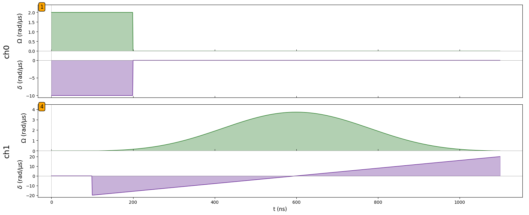
Now both channels have an initial target, so we can start building the sequence. Let’s start by creating a simple pulse with a constant Rabi frequency of 2 rad/µs and a constant detuning of -10 rad/µs that lasts 200 ns.

simple_pulse = pulser.Pulse.ConstantPulse(200, 2, -10, 0)

Let’s add this pulse to 'ch0':

seq.add(simple_pulse, "ch0")

Now, say we want to idle 'ch1' for 100 ns while 'ch0' is doing its pulse. We do that by calling:

seq.delay(100, "ch1")

Next, we want to create a more complex pulse to add to 'ch1', where the amplitude and the detuning are not constant. To do that, we use Waveforms:

duration = 1000
amp_wf = pulser.BlackmanWaveform(
    duration, np.pi / 2
)  # Duration: 1000 ns, Area: pi/2
detuning_wf = pulser.RampWaveform(
    duration, -20, 20
)  # Duration: 1000ns, linear sweep from -20 to 20 rad/µs

We can visualize a waveform by calling:

amp_wf.draw()

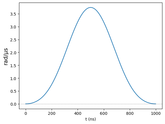
Also, it is often convenient to find the integral of a waveform, which can be obtain by calling:

amp_wf.integral  # dimensionless

1.5707963267948968

We then create the pulse with the waveforms instead of fixed values and we can also visualize it:

complex_pulse = pulser.Pulse(amp_wf, detuning_wf, phase=0)
complex_pulse.draw()

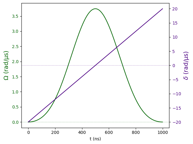
When we’re satisfied, we can then add it to a channel:

seq.add(complex_pulse, "ch1")

Let’s check the schedule to see how this is looking:

print(seq)

Channel: ch0
t: 0 | Initial targets: 1 | Phase Reference: 0.0
t: 0->200 | Pulse(Amp=2 rad/µs, Detuning=-10 rad/µs, Phase=0) | Targets: 1

Channel: ch1
t: 0 | Initial targets: 4 | Phase Reference: 0.0
t: 0->100 | Delay
t: 100->1100 | Pulse(Amp=Blackman(Area: 1.57), Detuning=Ramp(-20->20 rad/µs), Phase=0) | Targets: 4

We can also draw the sequence, for a more visual representation:

seq.draw()

Now, let’s see how the Sequence builder handles conflicts (i.e. two channels acting on the same qubit at once). We’re going to add a complex_pulseto 'ch0', but now we want to target it to qubit 4, which is the same target of 'ch1'.

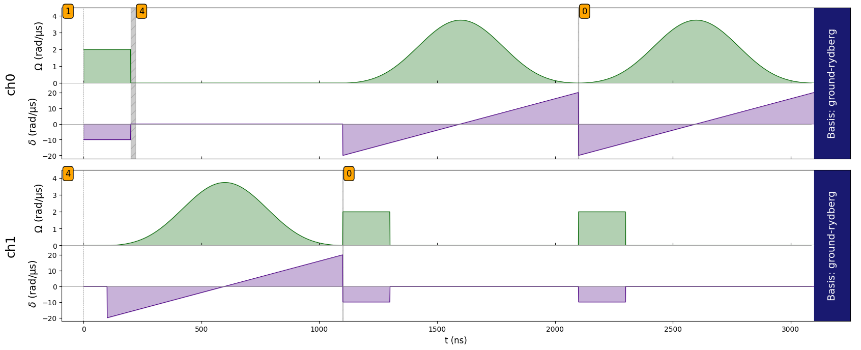
seq.target(4, "ch0")
seq.add(complex_pulse, "ch0")

print("Current Schedule:")
print(seq)
seq.draw()

Current Schedule:
Channel: ch0
t: 0 | Initial targets: 1 | Phase Reference: 0.0
t: 0->200 | Pulse(Amp=2 rad/µs, Detuning=-10 rad/µs, Phase=0) | Targets: 1
t: 200->220 | Target: 4 | Phase Reference: 0.0
t: 220->1100 | Delay
t: 1100->2100 | Pulse(Amp=Blackman(Area: 1.57), Detuning=Ramp(-20->20 rad/µs), Phase=0) | Targets: 4

Channel: ch1
t: 0 | Initial targets: 4 | Phase Reference: 0.0
t: 0->100 | Delay
t: 100->1100 | Pulse(Amp=Blackman(Area: 1.57), Detuning=Ramp(-20->20 rad/µs), Phase=0) | Targets: 4

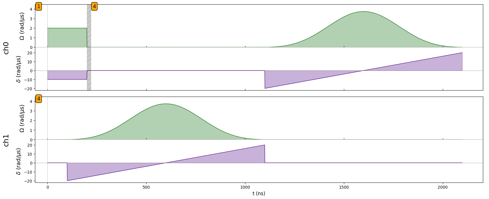
By looking at the current schedule, we can see that 'ch0' was delayed from ti=220 to tf=1100, and only then was the complex_pulse added. The reason for this is simple: it had to wait for the pulse on ch1, also targeted to qubit 4, to finish before it could apply its own. It behaved this way because, in Sequence.add there is a default argument protocol='min-delay.

Another protocol for pulse addition is wait-for-all, which makes the new pulse wait even if there is no conflict. Let’s remove the conflict and add two simple_pulses to ch1 with the different protocols to see how the compare.

seq.target(0, "ch1")
seq.add(simple_pulse, "ch1", protocol="min-delay")
seq.add(simple_pulse, "ch1", protocol="wait-for-all")

print("Current Schedule:")
print(seq)
seq.draw()

Current Schedule:
Channel: ch0
t: 0 | Initial targets: 1 | Phase Reference: 0.0
t: 0->200 | Pulse(Amp=2 rad/µs, Detuning=-10 rad/µs, Phase=0) | Targets: 1
t: 200->220 | Target: 4 | Phase Reference: 0.0
t: 220->1100 | Delay
t: 1100->2100 | Pulse(Amp=Blackman(Area: 1.57), Detuning=Ramp(-20->20 rad/µs), Phase=0) | Targets: 4

Channel: ch1
t: 0 | Initial targets: 4 | Phase Reference: 0.0
t: 0->100 | Delay
t: 100->1100 | Pulse(Amp=Blackman(Area: 1.57), Detuning=Ramp(-20->20 rad/µs), Phase=0) | Targets: 4
t: 1100->1100 | Target: 0 | Phase Reference: 0.0
t: 1100->1300 | Pulse(Amp=2 rad/µs, Detuning=-10 rad/µs, Phase=0) | Targets: 0
t: 1300->2100 | Delay
t: 2100->2300 | Pulse(Amp=2 rad/µs, Detuning=-10 rad/µs, Phase=0) | Targets: 0

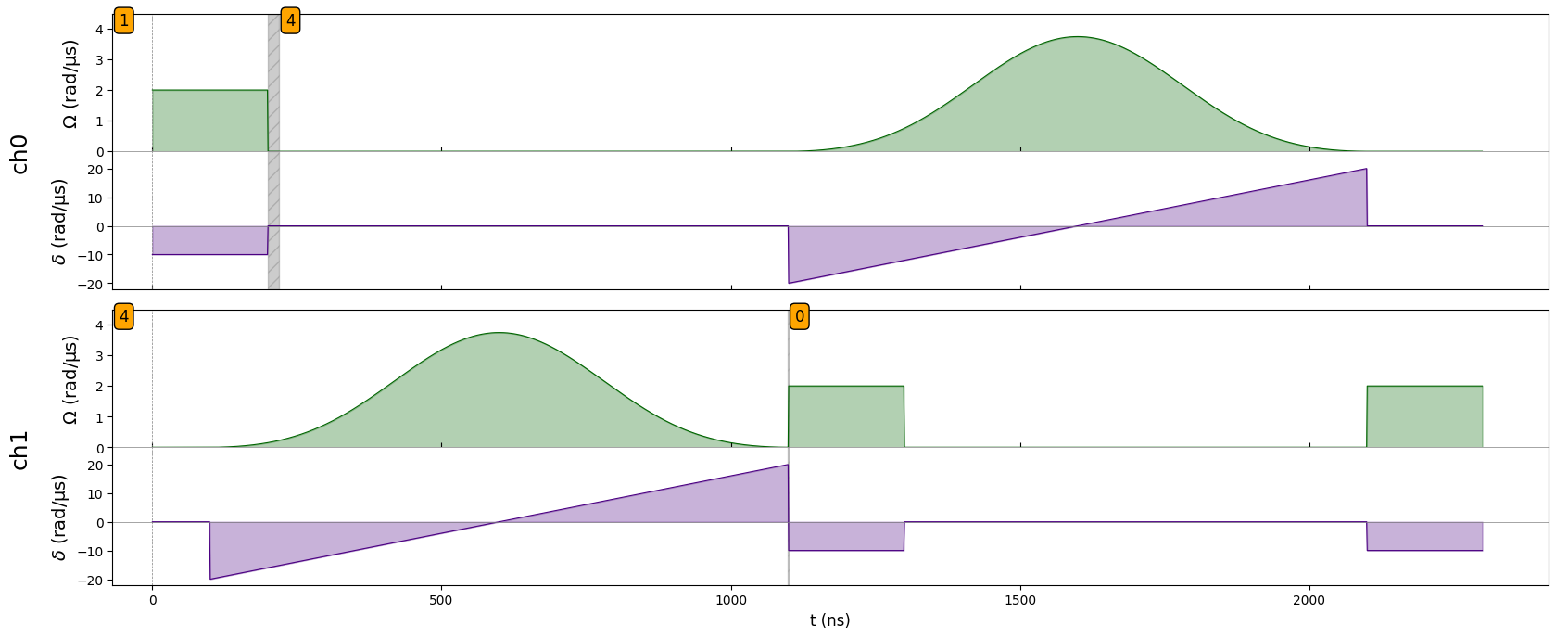
Because we removed the conflict by changing the target of ch1 to qubit 0, we see that the first pulse was added without delay from ti=1100 to tf=1300 (i.e. while complex_pulse is still running in ch0). However, once we changed to protocol='wait-for-all', there is now a delay (from ti=1300 to tf=2100) that idles ch1 until ch0is finished with its pulse, even though there was no conflict.

The third protocol is called 'no-delay' which, as the name implies, never delays the channel where the pulse is being added, even if that means introducing a conflict.

seq.target(0, "ch0")
seq.add(complex_pulse, "ch0", protocol="no-delay")

print("Current Schedule:")
print(seq)
seq.draw()

Current Schedule:
Channel: ch0
t: 0 | Initial targets: 1 | Phase Reference: 0.0
t: 0->200 | Pulse(Amp=2 rad/µs, Detuning=-10 rad/µs, Phase=0) | Targets: 1
t: 200->220 | Target: 4 | Phase Reference: 0.0
t: 220->1100 | Delay
t: 1100->2100 | Pulse(Amp=Blackman(Area: 1.57), Detuning=Ramp(-20->20 rad/µs), Phase=0) | Targets: 4
t: 2100->2100 | Target: 0 | Phase Reference: 0.0
t: 2100->3100 | Pulse(Amp=Blackman(Area: 1.57), Detuning=Ramp(-20->20 rad/µs), Phase=0) | Targets: 0

Channel: ch1
t: 0 | Initial targets: 4 | Phase Reference: 0.0
t: 0->100 | Delay
t: 100->1100 | Pulse(Amp=Blackman(Area: 1.57), Detuning=Ramp(-20->20 rad/µs), Phase=0) | Targets: 4
t: 1100->1100 | Target: 0 | Phase Reference: 0.0
t: 1100->1300 | Pulse(Amp=2 rad/µs, Detuning=-10 rad/µs, Phase=0) | Targets: 0
t: 1300->2100 | Delay
t: 2100->2300 | Pulse(Amp=2 rad/µs, Detuning=-10 rad/µs, Phase=0) | Targets: 0

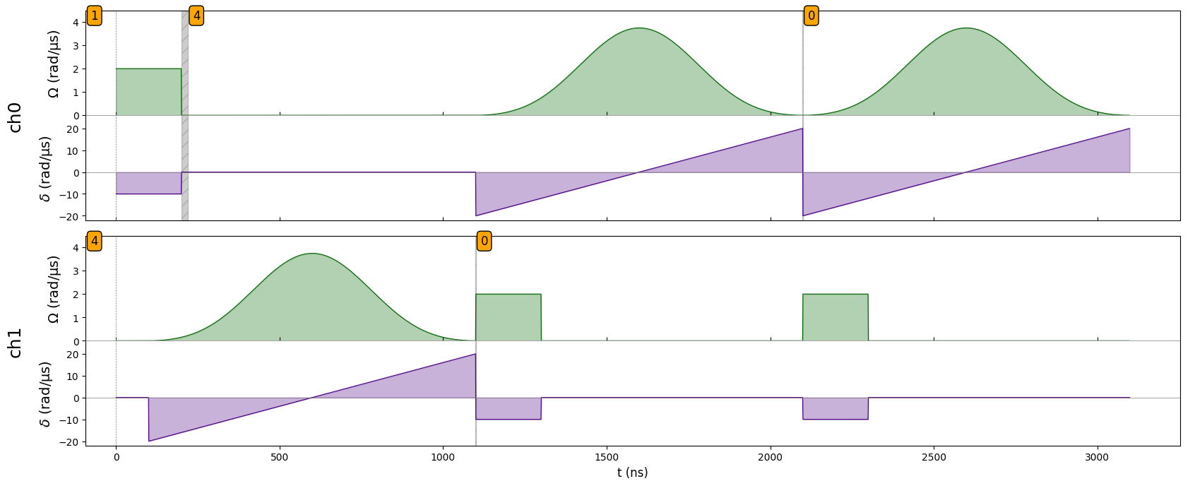
With this protocol, it is possible (though not advised), to create an overlap where multiple channels can be acting on the same qubit at the same time. Here, we can see that both act on qubit 0 from ti=2100 to tf=2300.

5. Measurement

To finish a sequence, we measure it. A measurement signals the end of a sequence, so after it no more changes are possible. We can measure a sequence by calling:

seq.measure(basis="ground-rydberg")

When measuring, one has to select the desired measurement basis. The availabe options depend on the device and can be consulted by calling:

DigitalAnalogDevice.supported_bases

{'digital', 'ground-rydberg'}

And so, we’ve obtained the final sequence!

seq.draw()