Conventions

States and Bases

Bases

A basis refers to a set of two eigenstates. The transition between these two states is said to be addressed by a channel that targets that basis. Namely:

Basis	Eigenstates	Channel type
ground-rydberg	\(|g\rangle,~|r\rangle\)	Rydberg
digital	\(|g\rangle,~|h\rangle\)	Raman
XY	\(|0\rangle,~|1\rangle\)	Microwave

Qutrit state

The qutrit state combines the basis states of the ground-rydberg and digital bases, which share the same ground state, \(|g\rangle\). This qutrit state comes into play in the digital approach, where the qubit state is encoded in \(|g\rangle\) and \(|h\rangle\) but then the Rydberg state \(|r\rangle\) is accessed in multi-qubit gates.

The qutrit state’s basis vectors are defined as:

\[|r\rangle = (1, 0, 0)^T,~~|g\rangle = (0, 1, 0)^T, ~~|h\rangle = (0, 0, 1)^T.\]

Qubit states

Warning

There is no implicit relationship between a state’s vector representation and its associated measurement value. To see the measurement value of a state for each measurement basis, see State Preparation and Measurement .

When using only the ground-rydberg or digital basis, the qutrit state is not needed and is thus reduced to a qubit state. This reduction is made simply by tracing-out the extra basis state, so we obtain

• ground-rydberg: \(|r\rangle = (1, 0)^T,~~|g\rangle = (0, 1)^T\)

• digital: \(|g\rangle = (1, 0)^T,~~|h\rangle = (0, 1)^T\)

On the other hand, the XY basis uses an independent set of qubit states that are labelled \(|0\rangle\) and \(|1\rangle\) and follow the standard convention:

• XY: \(|0\rangle = (1, 0)^T,~~|1\rangle = (0, 1)^T\)

Multi-partite states

The combined quantum state of multiple atoms respects their order in the Register. For a register with ordered atoms (q0, q1, q2, ..., qn), the full quantum state will be

\[|q_0, q_1, q_2, ...\rangle = |q_0\rangle \otimes |q_1\rangle \otimes |q_2\rangle \otimes ... \otimes |q_n\rangle\]

Note

The atoms may be labelled arbitrarily without any inherent order, it’s only the order with which they are stored in the Register (as returned by Register.qubit_ids) that matters .

State Preparation and Measurement

Initial State and Measurement Conventions

Basis	Initial state	Measurement
ground-rydberg	\(|g\rangle\)	\(|r\rangle \rightarrow 1\) \(|g\rangle,|h\rangle \rightarrow 0\)
digital	\(|g\rangle\)	\(|h\rangle \rightarrow 1\) \(|g\rangle,|r\rangle \rightarrow 0\)
XY	\(|0\rangle\)	\(|1\rangle \rightarrow 1\) \(|0\rangle \rightarrow 0\)

Measurement samples order

Measurement samples are returned as a sequence of 0s and 1s, in the same order as the atoms in the Register and in the multi-partite state.

For example, a four-qutrit state \(|q_0, q_1, q_2, q_3\rangle\) that’s projected onto \(|g, r, h, r\rangle\) when measured will record a count to sample

• 0101, if measured in the ground-rydberg basis

• 0010, if measured in the digital basis

Hamiltonians

Independently of the mode of operation, the Hamiltonian describing the system can be written as

\[H(t) = \sum_i \left (H^D_i(t) + \sum_{j<i}H^\text{int}_{ij} \right),\]

where \(H^D_i\) is the driving Hamiltonian for atom \(i\) and \(H^\text{int}_{ij}\) is the interaction Hamiltonian between atoms \(i\) and \(j\). Note that, if multiple basis are addressed, there will be a corresponding driving Hamiltonian for each transition.

Driving Hamiltonian

The driving Hamiltonian describes the coherent excitation of an individual atom between two energies levels, \(|a\rangle\) and \(|b\rangle\), with Rabi frequency \(\Omega(t)\), detuning \(\delta(t)\) and phase \(\phi(t)\).

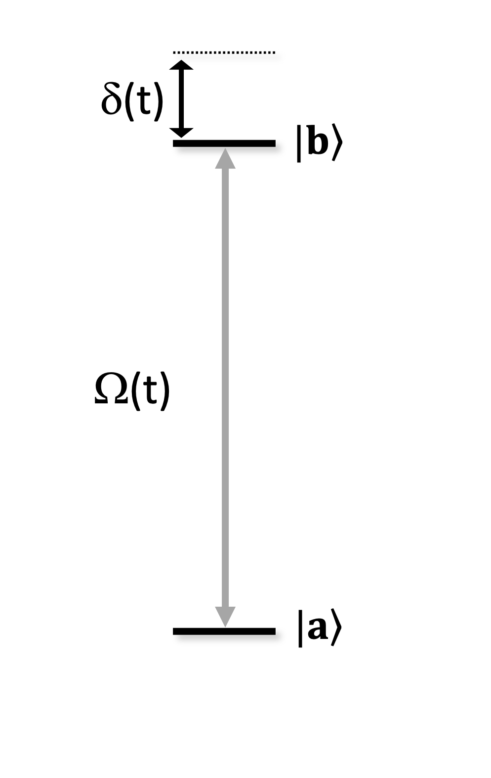
The coherent excitation is driven between a lower energy level, \(|a\rangle\), and a higher energy level, \(|b\rangle\), with Rabi frequency \(\Omega(t)\) and detuning \(\delta(t)\).

Warning

In this form, the Hamiltonian is independent of the state vector representation of each basis state, but it still assumes that \(|b\rangle\) has a higher energy than \(|a\rangle\).

\[H^D(t) / \hbar = \frac{\Omega(t)}{2} e^{-i\phi(t)} |a\rangle\langle b| + \frac{\Omega(t)}{2} e^{i\phi(t)} |b\rangle\langle a| - \delta(t) |b\rangle\langle b|\]

Pauli matrix form

A more conventional representation of the driving Hamiltonian uses Pauli operators instead of projectors. However, this form now depends on the state vector definition of \(|a\rangle\) and \(|b\rangle\).

Pulser’s state-vector definition

In Pulser, we consistently define the state vectors according to their relative energy. In this way we have, for any given basis, that

\[|b\rangle = (1, 0)^T,~~|a\rangle = (0, 1)^T\]

Thus, the Pauli and excited state occupation operators are defined as

\[\begin{split}\hat{\sigma}^x = |a\rangle\langle b| + |b\rangle\langle a|, \\ \hat{\sigma}^y = i|a\rangle\langle b| - i|b\rangle\langle a|, \\ \hat{\sigma}^z = |b\rangle\langle b| - |a\rangle\langle a| \\ \hat{n} = |b\rangle\langle b| = (1 + \sigma_z) / 2\end{split}\]

and the driving Hamiltonian takes the form

\[H^D(t) / \hbar = \frac{\Omega(t)}{2} \cos\phi(t) \hat{\sigma}^x - \frac{\Omega(t)}{2} \sin\phi(t) \hat{\sigma}^y - \delta(t) \hat{n}\]

Alternative state-vector definition

Outside of Pulser, the alternative definition for the basis state vectors might be taken:

\[|a\rangle = (1, 0)^T,~~|b\rangle = (0, 1)^T\]

This changes the operators and Hamiltonian definitions, as rewriten below with highlighted differences.

\[\begin{split}\hat{\sigma}^x = |a\rangle\langle b| + |b\rangle\langle a|, \\ \hat{\sigma}^y = \textcolor{red}{-}i|a\rangle\langle b| \textcolor{red}{+}i|b\rangle\langle a|, \\ \hat{\sigma}^z = \textcolor{red}{-}|b\rangle\langle b| \textcolor{red}{+} |a\rangle\langle a| \\ \hat{n} = |b\rangle\langle b| = (1 \textcolor{red}{-} \sigma_z) / 2\end{split}\]

\[H^D(t) / \hbar = \frac{\Omega(t)}{2} \cos\phi(t) \hat{\sigma}^x \textcolor{red}{+}\frac{\Omega(t)}{2} \sin\phi(t) \hat{\sigma}^y - \delta(t) \hat{n}\]

Note

A common case for the use of this alternative definition arises when trying to reconcile the basis states of the ground-rydberg basis (where \(|r\rangle\) is the higher energy level) with the computational-basis state-vector convention, thus ending up with

\[|0\rangle = |g\rangle = |a\rangle = (1, 0)^T,~~|1\rangle = |r\rangle = |b\rangle = (0, 1)^T\]

Interaction Hamiltonian

The interaction Hamiltonian depends on the states involved in the sequence. When working with the ground-rydberg and digital bases, atoms interact when they are in the Rydberg state \(|r\rangle\):

\[H^\text{int}_{ij} = \frac{C_6}{R_{ij}^6} \hat{n}_i \hat{n}_j\]

where \(\hat{n}_i = |r\rangle\langle r|_i\) (the projector of atom \(i\) onto the Rydberg state), \(R_{ij}^6\) is the distance between atoms \(i\) and \(j\) and \(C_6\) is a coefficient depending on the specific Rydberg level of \(|r\rangle\).

On the other hand, with the two Rydberg states of the XY basis, the interaction Hamiltonian takes the form

\[H^\text{int}_{ij} = \frac{C_3}{R_{ij}^3} (\hat{\sigma}_i^{+}\hat{\sigma}_j^{-} + \hat{\sigma}_i^{-}\hat{\sigma}_j^{+})\]

where \(C_3\) is a coefficient that depends on the chosen Ryberg states and

\[\hat{\sigma}_i^{+} = |1\rangle\langle 0|_i,~~~\hat{\sigma}_i^{-} = |0\rangle\langle 1|_i\]

Note

The definitions given for both interaction Hamiltonians are independent of the chosen state vector convention.