XY Spin Chain

We introduce here a new mode of interaction between the atoms driven by the dipole-dipole interaction. This mode is called the XY mode. The interaction hamiltonian of a system of \(N\) qubits is now given by

\[H_{XY} = \sum_{i=1}^N\sum_{j<i} \frac{C_3}{R_{ij}^3}(\sigma^+_i \sigma^-_j + \sigma^-_i \sigma^+_j)\]

where \(\sigma^{±} = (\sigma^x ± i\sigma^y)/2\), \(R_{ij}\) is the distance between atom \(i\) and atom \(j\), and \(C_3\) is a coefficient dependent on the device and taken as \(\frac{C_3}{\hbar} = 3700 \mu m^3/\mu s\) for the MockDevice.

The final hamiltonian of the system is

\[H= \sum_{i=1}^N \frac{\hbar\Omega}{2} \sigma_i^x - \sum_{i=1}^N \frac{\hbar \delta}{2} \sigma_i^z+H_{XY}.\]

The Rydberg states involved are different from the ones of the Ising interaction, they are \(|0\rangle = |62D_{3/2}, m_j=3/2 \rangle\) and \(|1\rangle = |63P_{1/2}, m_j=1/2 \rangle\).

More details on the XY mode can be found in the following reference: Barredo et al. 2014

import numpy as np
import matplotlib.pyplot as plt
import qutip

import pulser
from pulser import Pulse, Sequence, Register
from pulser_simulation import QutipEmulator
from pulser.devices import MockDevice
from pulser.waveforms import BlackmanWaveform

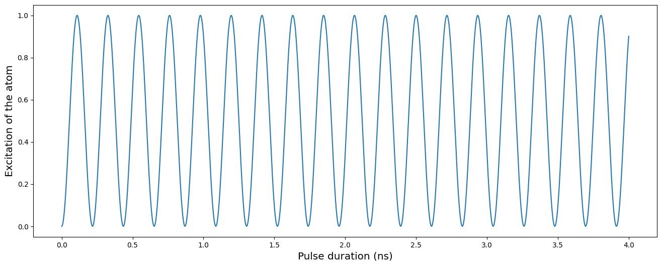
Rabi oscillations of 1 atom

We start by showing Rabi oscillation in the XY mode in the case of a unique atom as shown in the figure 1 (c) of the reference. In a similar way as the Ising mode, the atom will oscillate between the two energy levels. The XY mode is only available in the mw_global channel. We initialize the register and instantiate the channel.

coords = np.array([[0, 0]])
qubits = dict(enumerate(coords))

reg = Register(qubits)
seq = Sequence(reg, MockDevice)
seq.declare_channel("MW", "mw_global")

We then add a simple constant rabi pulse of amplitude \(2\pi \times 4.6\) MHz and run the simulation. The measurement is necessarily done in the XY basis.

simple_pulse = Pulse.ConstantPulse(4000, 2 * np.pi * 4.6, 0, 0)
seq.add(simple_pulse, "MW")
seq.measure(basis="XY")

sim = QutipEmulator.from_sequence(seq)

results = sim.run(progress_bar=True, nsteps=5000)

10.0%. Run time:   0.03s. Est. time left: 00:00:00:00

20.0%. Run time:   0.07s. Est. time left: 00:00:00:00

30.0%. Run time:   0.10s. Est. time left: 00:00:00:00

40.0%. Run time:   0.14s. Est. time left: 00:00:00:00

50.0%. Run time:   0.17s. Est. time left: 00:00:00:00

60.0%. Run time:   0.21s. Est. time left: 00:00:00:00

70.0%. Run time:   0.25s. Est. time left: 00:00:00:00

80.0%. Run time:   0.28s. Est. time left: 00:00:00:00

90.0%. Run time:   0.32s. Est. time left: 00:00:00:00

Total run time:   0.35s

We plot the expectation of the excitation of the atom over the time.

def excitation(j, total_sites):
    """The |1><1| projector operator on site j."""
    prod = [qutip.qeye(2) for _ in range(total_sites)]
    prod[j] = (qutip.qeye(2) - qutip.sigmaz()) / 2
    return qutip.tensor(prod)


excited = excitation(0, 1)
plt.figure(figsize=[16, 6])
results.plot(excited)
plt.xlabel("Pulse duration (ns)", fontsize="x-large")
plt.ylabel("Excitation of the atom", fontsize="x-large")
plt.show()

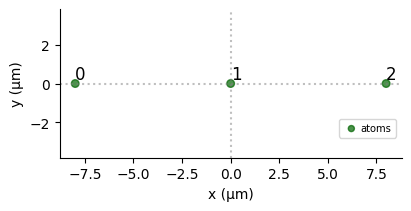
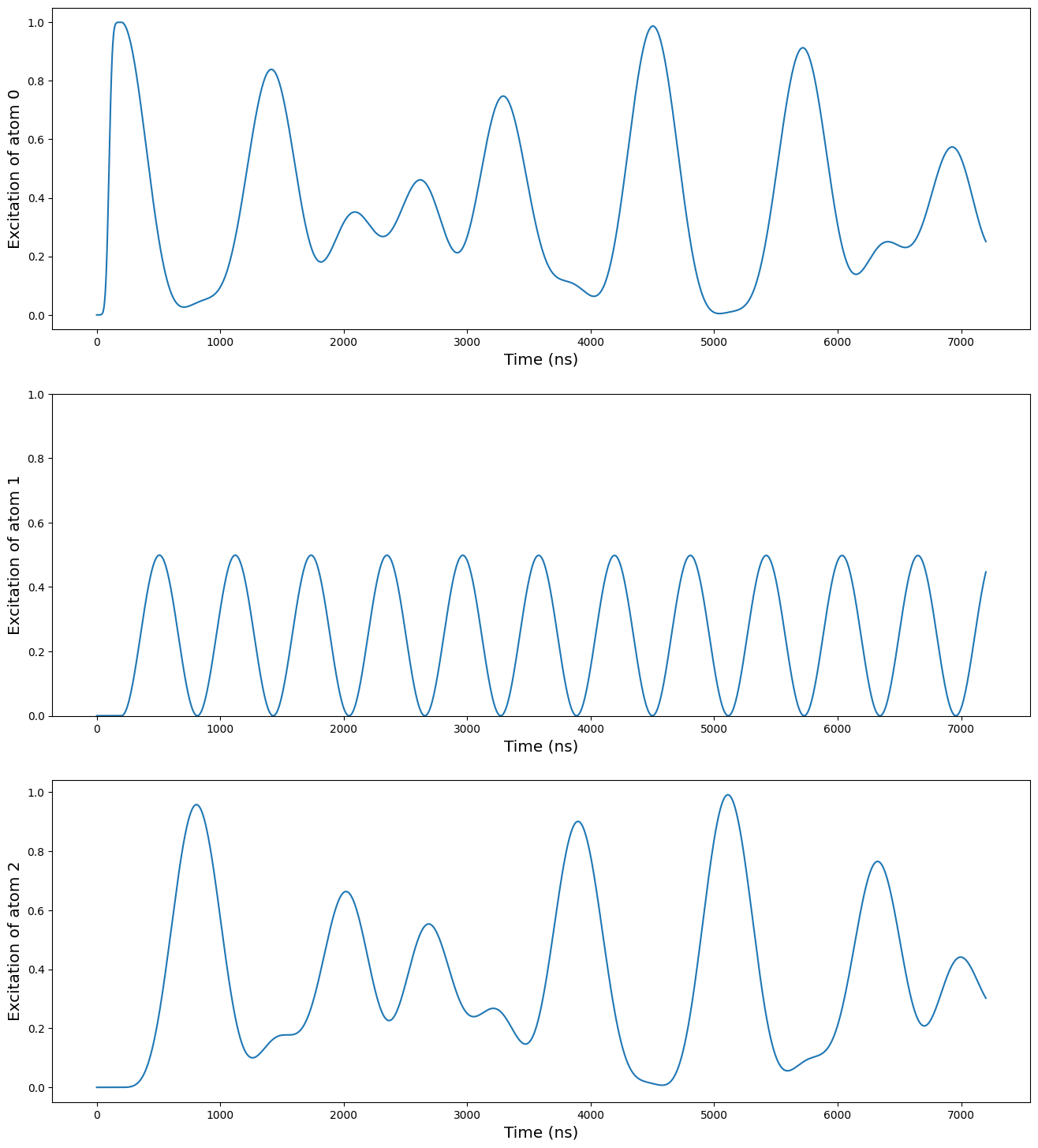
Spin chain of 3 atoms

We now simulate the free evolution of a spin chain of 3 atoms, starting with 1 excitation in the initial state \(|100\rangle\) as shown in the figure 3 (c) of the reference.

coords = np.array([[-8.0, 0], [0, 0], [8.0, 0]])
qubits = dict(enumerate(coords))

reg = Register(qubits)
seq = Sequence(reg, MockDevice)
seq.declare_channel("ch0", "mw_global")
reg.draw()

# State preparation using SLM mask
masked_qubits = [1, 2]
seq.config_slm_mask(masked_qubits)
masked_pulse = Pulse.ConstantDetuning(BlackmanWaveform(200, np.pi), 0, 0)
seq.add(masked_pulse, "ch0")

# Simulation pulse
simple_pulse = Pulse.ConstantPulse(7000, 0, 0, 0)
seq.add(simple_pulse, "ch0")
seq.measure(basis="XY")

sim = QutipEmulator.from_sequence(seq, sampling_rate=1)
results = sim.run(nsteps=5000)

excited_list = [excitation(j, 3) for j in range(3)]

expectations = results.expect(excited_list)

plt.figure(figsize=[16, 18])
plt.subplot(311)
plt.plot(expectations[0])
plt.ylabel("Excitation of atom 0", fontsize="x-large")
plt.xlabel("Time (ns)", fontsize="x-large")
plt.subplot(312)
plt.plot(expectations[1])
plt.ylabel("Excitation of atom 1", fontsize="x-large")
plt.xlabel("Time (ns)", fontsize="x-large")
plt.ylim([0, 1])
plt.subplot(313)
plt.plot(expectations[2])
plt.ylabel("Excitation of atom 2", fontsize="x-large")
plt.xlabel("Time (ns)", fontsize="x-large")
plt.show()

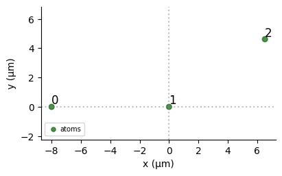
External field and angular dependency

An external magnetic field can be added to the experiment, and will modify the hamiltonian. The XY Hamiltonian is then

\[H_{XY} = \sum_{i=1}^N\sum_{j<i} \frac{C_3[1 - 3\text{cos}^2(\theta_{ij})]}{R_{ij}^3}(\sigma^+_i \sigma^-_j + \sigma^-_i \sigma^+_j)\]

where \(\theta_{ij}\) is the angle between the vector of the two atoms and the external field as shown on the figure below.

We add an external field along the Y axis, and we put the qubit 2 at the angle such that \(\text{cos}^2(\theta_{12}) = 1/3\), and the interaction between the qubits 1 and 2 cancels out. This is done by the method set_magnetic_fieldfrom the Sequence.

This is the principle that enables to create topological phases on long chain of atoms.

coords = np.array([[-1.0, 0], [0, 0], [np.sqrt(2 / 3), np.sqrt(1 / 3)]]) * 8.0
qubits = dict(enumerate(coords))

reg = Register(qubits)
seq = Sequence(reg, MockDevice)
seq.declare_channel("ch0", "mw_global")
seq.set_magnetic_field(0.0, 1.0, 0)
reg.draw()

We then simulate again the free evolution from the initial state \(|100\rangle\).

# State preparation using SLM mask
masked_qubits = [1, 2]
seq.config_slm_mask(masked_qubits)
masked_pulse = Pulse.ConstantDetuning(BlackmanWaveform(200, np.pi), 0, 0)
seq.add(masked_pulse, "ch0")

# Simulation pulse
simple_pulse = Pulse.ConstantPulse(7000, 0, 0, 0)
seq.add(simple_pulse, "ch0")
seq.measure(basis="XY")

sim = QutipEmulator.from_sequence(seq, sampling_rate=1)
results = sim.run(progress_bar=True, nsteps=5000)

10.0%. Run time:   0.06s. Est. time left: 00:00:00:00

20.0%. Run time:   0.13s. Est. time left: 00:00:00:00

30.0%. Run time:   0.19s. Est. time left: 00:00:00:00

40.0%. Run time:   0.27s. Est. time left: 00:00:00:00

50.0%. Run time:   0.35s. Est. time left: 00:00:00:00

60.0%. Run time:   0.42s. Est. time left: 00:00:00:00

70.0%. Run time:   0.50s. Est. time left: 00:00:00:00

80.0%. Run time:   0.57s. Est. time left: 00:00:00:00

90.0%. Run time:   0.65s. Est. time left: 00:00:00:00

Total run time:   0.73s

excited_list = [excitation(j, 3) for j in range(3)]

expectations = results.expect(excited_list)

plt.figure(figsize=[16, 18])
plt.subplot(311)
plt.plot(expectations[0])
plt.ylabel("Excitation of atom 0", fontsize="x-large")
plt.xlabel("Time ($\mu$s)", fontsize="x-large")
plt.ylim([0, 1])
plt.subplot(312)
plt.plot(expectations[1])
plt.ylabel("Excitation of atom 1", fontsize="x-large")
plt.xlabel("Time ($\mu$s)", fontsize="x-large")
plt.ylim([0, 1])
plt.subplot(313)
plt.plot(expectations[2])
plt.ylabel("Excitation of atom 2", fontsize="x-large")
plt.xlabel("Time ($\mu$s)", fontsize="x-large")
plt.ylim([0, 1])
plt.show()

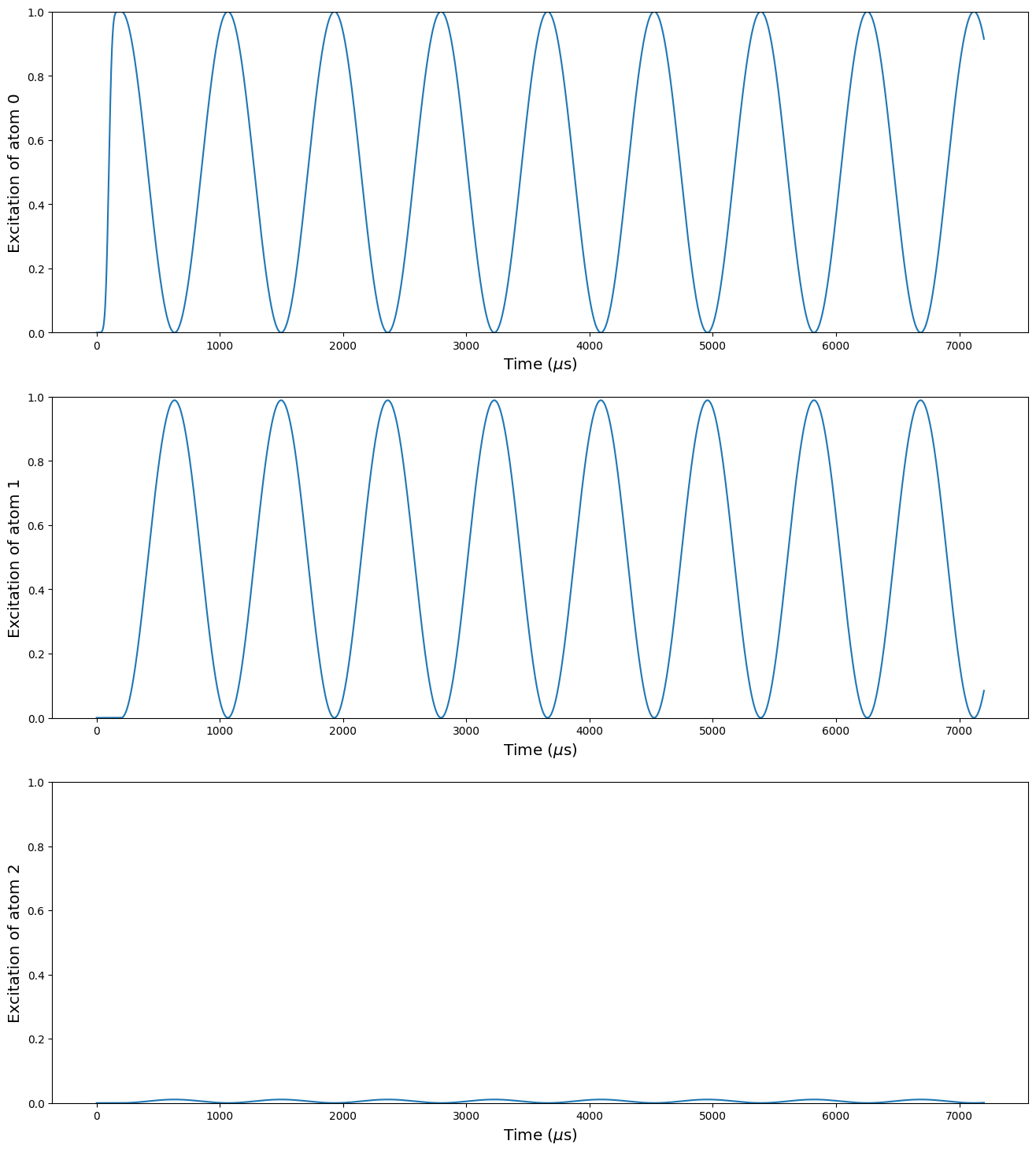
We can see there that there is almost no excitation in the qubit 2. It still remains some because the interaction between the qubits 0 and 2 is not completely negligible.