Local Addressability with DMM

import numpy as np

from dataclasses import replace

from matplotlib import pyplot as plt

from pulser.devices import WeightedAnalogDevice
from pulser.register import Register
from pulser.register.register_layout import RegisterLayout
from pulser.register.mappable_reg import MappableRegister
from pulser.sampler import sampler
from pulser.sequence import Sequence
from pulser.pulse import Pulse
from pulser.waveforms import ConstantWaveform, RampWaveform

Introduction

Even when working with global addressing channels, the detuning of individual qubits can be addressed locally by using a specific channel named the Detuning Map Modulator or DMM.

This Channel applies a Global pulse of zero amplitude and negative detuning on a DetuningMap. The DetuningMap consists of a set of weights on specific sites that dictate the proportion of detuning applied by the DMM each site receives.

This modulation of the DetuningMap by the DMM Channel is equivalent to adding a term \(-\hbar\sum_{k}\epsilon_{k}\delta_{DMM}(t)|r\rangle\langle r|_k\) to the Ising Hamiltonian. Here, \(\delta_{DMM}(t)\) is the detuning applied on the DMM, and \(\epsilon_k\) are the weights defined in the DetuningMap for each atom.

The inclusion of this term results in the Weighted-Analog Ising Hamiltonian:

\[\frac{H(t)}{\hbar} = \sum_{k=1}^N \left (\frac{\Omega(t)}{2} e^{-i\phi(t)} |g\rangle\langle r|_k + \frac{\Omega(t)}{2} e^{i\phi(t)} |r\rangle\langle g|_k - \left[\delta(t)\mathbf{+\epsilon_k\delta_{DMM}(t)}\right] |r\rangle\langle r|_k + \sum_{j<k}\frac{C_6}{\hbar R_{kj}^6} \hat{n}_k \hat{n}_j \right)\]

Define a Detuning Map

A DetuningMap associates a set of locations with a set of weights. The locations are the trap coordinates to address and the weights \((\epsilon_i)_i\) have to be between 0 and 1.

trap_coordinates = [(0.0, 0.0), (0.0, 5.0), (5.0, 0.0), (5.0, 5.0)]
weights = [1.0, 0.5, 0.5, 0]  # between 0 and 1

The DetuningMap can be defined from a RegisterLayout, a Register or a MappableRegister by using the define_detuning_map method. All it takes is a mapping between trap/qubit IDs and weights.

register_layout = RegisterLayout(trap_coordinates)
detuning_map = register_layout.define_detuning_map(
    {i: weights[i] for i in range(4)}  # mapping between trap IDs and weights
)

map_reg = MappableRegister(register_layout)
det_map_from_map_reg = map_reg.define_detuning_map(
    {i: weights[i] for i in range(4)}  # mapping between trap IDs and weights
)

register = Register.from_coordinates(
    trap_coordinates, center=False, prefix="q"
)
det_map_from_reg = register.define_detuning_map(
    {
        f"q{i}": weights[i] for i in range(4)
    }  # mapping between qubit IDs and weights
)

detuning_map.draw(labels=[0, 1, 2, 3])
assert detuning_map == det_map_from_map_reg
assert detuning_map == det_map_from_reg

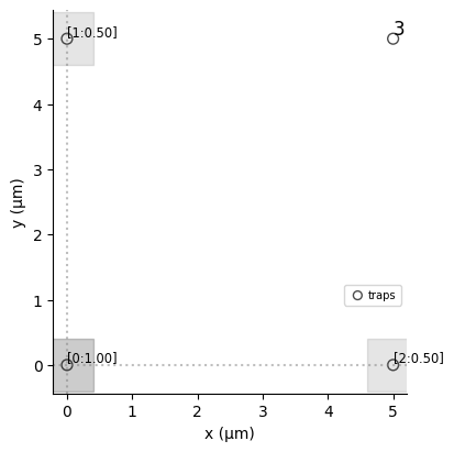
The traps are represented by a grey dot and highlighted by a grey square, whose shade is proportional to the value of the associated weight. It is possible to display the value of the weights by specifying a list of labels. If the weight is null then no DMM is applied: the atom is not highlighted by a grey square and the value of the weight is not shown when labels are specified.

DMM Channel and Device

A DMM Channel is a Channel that accepts pulses of zero amplitude and detuning below 0 and above:

• bottom_detuning for each site.

• total_bottom_detuning for the total detuning distributed among the atoms.

The DMM channels are defined separately from the other channels of the device. They are defined as a list in dmm_objects. They can be accessed via the property dmm_channels of the device, where an ID is automatically associated to each DMM with the format dmm_{index of appearance in dmm_objects}.

pulser.devices.WeightedAnalogDevice is an example of a device containing one DMM channel, accessible via the ID dmm_0:

print(WeightedAnalogDevice.dmm_channels)

{'dmm_0': DMM(clock_period=4, min_duration=16, max_duration=100000000, mod_bandwidth=22, eom_config=None, bottom_detuning=-62.83185307179586, total_bottom_detuning=-6283.185307179586, min_avg_abs_detuning=0.6283185307179586)}

DMM in a Sequence

In a Sequence defined with a Device having dmm_objects, the DMM channels can be configured using config_detuning_map. This configuration associates a DMM - referenced by dmm_id in the Device- with a DetuningMap, under a dmm_name in the Sequence.

seq = Sequence(register, WeightedAnalogDevice)
seq.config_detuning_map(detuning_map, "dmm_0")
print(seq.declared_channels)

{'dmm_0': DMM(clock_period=4, min_duration=16, max_duration=100000000, mod_bandwidth=22, eom_config=None, bottom_detuning=-62.83185307179586, total_bottom_detuning=-6283.185307179586, min_avg_abs_detuning=0.6283185307179586)}

The dmm_name in the Sequence is generated automatically. It is dmm_id if the DMM labeled dmm_id in the Device hasn’t been configured yet. The same dmm_id can be configured multiple times only if we use a VirtualDevice with reusable_channels=True. In this case, the dmm_name would take the suffix _{number of times dmm_id has been declared so far}. For instance, if we have configured the DMM labeled dmm_0 once, configuring it a second time would declare a new DMM with name dmm_0_1.

Let’s now apply a global detuning on the detuning map. This is done by calling add_dmm_detuning and providing a waveform (the detuning \(\Delta(t)\) to modulate the DetuningMap with) and the dmm_name to use (provides the DetuningMap and checks that \(\Delta(t)\) is in agreement with the characteristics of the corresponding DMM).

seq.add_dmm_detuning(ConstantWaveform(100, -10), "dmm_0")
seq.draw(draw_detuning_maps=True)

Once a detuning map is configured, it is no longer possible to define a Microwave channel. However, it is possible to declare Rydberg and Raman channels. Let’s declare a Rydberg.Global channel in our sequence.

seq.declare_channel("ryd_glob", "rydberg_global")

Be careful with the protocols that are used to add the pulses to Channels and DMM:

• The default protocol to add a waveform to a DMM is "no-delay", meaning that it will be added straight after the last pulse, without caring about the other channels. As an example, the second waveform added to dmm_0 below starts at the end of the first waveform added to dmm_0 (at t=100 ns) and not after the pulse added to the Global Rydberg channel (which finishes at t=152 ns), which would have been the case with the protocol "min_delay". The protocol can be changed to other values by defining the protocol argument.

• The protocol to add a pulse to a Rydberg or a Raman channel is "min-delay", meaning that the pulse will by default be added after the end of the pulse of a DMM. It can be switched to "no-delay".

seq.add(
    Pulse.ConstantPulse(152, 10, 2.5, 0), "ryd_glob", protocol="no-delay"
)  # added at the beginning with protocol "no delay"
seq.add_dmm_detuning(RampWaveform(200, -10, 0), "dmm_0")  # added at t=100
seq.add(
    Pulse.ConstantPulse(100, 5, 0, 0), "ryd_glob", protocol="no-delay"
)  # added at t=150 after the last pulse on `ryd_glob`, with protocol "no-delay"
seq.draw()

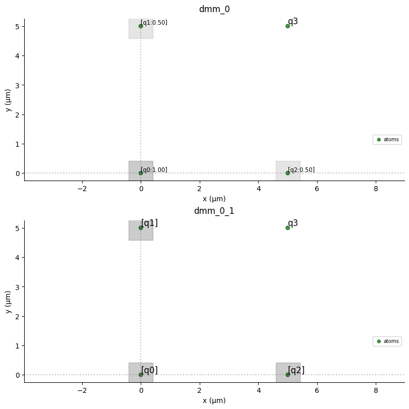
It is possible to display the amplitude and detuning per qubits, by setting to True the arguments draw_qubit_amp and draw_qubit_det. This adds two plots after the drawing of the sequence. The first one shows the evolution of these quantities along time for groups of qubits experiencing the same amplitude or detuning. The second represents these group of qubits on a register.

seq.draw(
    mode="input+output",  # "input" only shows input signals, "input+output"
    draw_qubit_det=True,
    draw_qubit_amp=True,
)

You can see that by combining a global pulse with a positive detuning and a pulse on the DMM channel, it is possible to have positive local detuning (see the detuning on q3 from t=0 to t=152 ns).

It can also be noted that from t=100 ns to t=300 ns, the local detuning is defined by the detuning ramp applied on detuning_map, hence it is locally a detuning ramp, going to 0 with a slope defined by the weight of detuning_map on each atom. This is why the detuning on q3 during this duration is equal to the one of the global Rydberg’s channel and that q1 and q2 have the same local detuning (they are part of the same “target” group for the detuning).

In action:

Local addressability can be used to find the Maximally Weighted Independent Set (MWIS) of a graph.