Simulation of XYZ spin models using Floquet engineering in XY mode

import numpy as np
import matplotlib
import matplotlib.pyplot as plt
import qutip

import pulser
from pulser import Pulse, Sequence, Register
from pulser_simulation import QutipEmulator
from pulser.devices import MockDevice
from pulser.waveforms import BlackmanWaveform

In this notebook, we will reproduce some results of “Microwave-engineering of programmable XXZ Hamiltonians in arrays of Rydberg atoms”, P. Scholl, et. al., https://arxiv.org/pdf/2107.14459.pdf.

Floquet Engineering on two atoms

We start by considering the dynamics of two interacting atoms under \(H_{XXZ}\). To demonstrate the dynamically tunable aspect of the microwave engineering, we change the Hamiltonian during the evolution of the system. More specifically, we start from \(|\rightarrow \rightarrow \rangle_y\), let the atoms evolve under \(H_{XX}\) and apply a microwave pulse sequence between \(0.9\mu s\) and \(1.2\mu s\) only.

Let us first define our \(\pm X\) and \(\pm Y\) pulses.

# Times are in ns
t_pulse = 26

X_pulse = Pulse.ConstantDetuning(BlackmanWaveform(t_pulse, np.pi / 2.0), 0, 0)
Y_pulse = Pulse.ConstantDetuning(
    BlackmanWaveform(t_pulse, np.pi / 2.0), 0, -np.pi / 2
)
mX_pulse = Pulse.ConstantDetuning(
    BlackmanWaveform(t_pulse, np.pi / 2.0), 0, np.pi
)
mY_pulse = Pulse.ConstantDetuning(
    BlackmanWaveform(t_pulse, np.pi / 2.0), 0, np.pi / 2
)

Let’s also define a function to add the pulses during one cycle.

def Floquet_XXZ_cycles(n_cycles, tau_1, tau_2, t_pulse):
    t_half = t_pulse / 2.0
    tau_3 = tau_2
    tc = 4 * tau_2 + 2 * tau_1
    for _ in range(n_cycles):
        seq.delay(tau_1 - t_half, "MW")
        seq.add(X_pulse, "MW")
        seq.delay(tau_2 - 2 * t_half, "MW")
        seq.add(mY_pulse, "MW")
        seq.delay(2 * tau_3 - 2 * t_half, "MW")
        seq.add(Y_pulse, "MW")
        seq.delay(tau_2 - 2 * t_half, "MW")
        seq.add(mX_pulse, "MW")
        seq.delay(tau_1 - t_half, "MW")

We are ready to start building our sequence.

# We take two atoms distant by 10 ums.
coords = np.array([[0, 0], [10, 0]])
qubits = dict(enumerate(coords))
reg = Register(qubits)

seq = Sequence(reg, MockDevice)
seq.declare_channel("MW", "mw_global")
seq.set_magnetic_field(0.0, 0.0, 1.0)

tc = 300
seq.delay(3 * tc, "MW")
Floquet_XXZ_cycles(4, tc / 6.0, tc / 6.0, t_pulse)
seq.delay(6 * tc, "MW")

# Here are our evaluation times
t_list = []
for p in range(13):
    t_list.append(tc / 1000.0 * p)

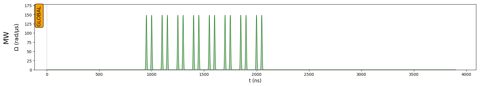
Let’s draw the sequence, to see that the microwave engineering only happens between \(900 ns\) and \(2100 ns\), which corresponds to \(H_{XX} \to H_{XXX}\). During that period, the total y-magnetization \(\langle \sigma^y_1 + \sigma^y_2 \rangle\) is expected to be frozen, as this quantity commutes with \(H_{XXX}\).

seq.draw()

sim = QutipEmulator.from_sequence(
    seq, sampling_rate=1.0, config=None, evaluation_times=t_list
)
psi_y = (qutip.basis(2, 0) + 1j * qutip.basis(2, 1)).unit()
sim.set_initial_state(qutip.tensor(psi_y, psi_y))
res = sim.run()

sy = qutip.sigmay()
Id = qutip.qeye(2)
Sigma_y = (qutip.tensor(sy, Id) + qutip.tensor(Id, sy)) / 2.0
Sigma_y_res = res.expect([Sigma_y])

plt.figure()

# Showing the Hamiltonian engineering period.
line1 = 0.9
line2 = 2.1
plt.axvspan(line1, line2, alpha=0.1, color="grey")
plt.text(1.0, 0.5, r"$H_{XX} \to H_{XXX}$", fontsize=14)

plt.plot(sim.evaluation_times, Sigma_y_res[0], "o")
plt.xlabel(r"Time [µs]", fontsize=16)
plt.ylabel(rf"$ (\langle \sigma_1^y + \sigma_2^y \rangle)/2$", fontsize=16)
plt.show()

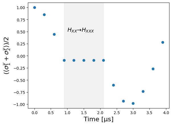
Note that one cannot directly measure off diagonal elements of the density matrix experimentally. To be able to measure \(\langle \sigma^y_1 + \sigma^y_2 \rangle\), one would need to first apply a rotation on the atoms (equivalent to changing the basis) and then measure the population.

Domain-wall dynamics

Now, we will look at the dynamics of the system under \(H_{XX2Z}\) when starting in a Domain-Wall (DW) state \(|\psi_0\rangle = |\uparrow \uparrow \uparrow \uparrow \uparrow \downarrow \downarrow \downarrow \downarrow \downarrow\rangle \equiv |0000011111\rangle\), for two distinct geometries : open boundary conditions (OBC) and periodic boundary conditions (PBC). In the case of \(H_{XX2Z}\), only 2 pulses per Floquet cycle are required, as the \(X\) and \(-X\) pulses cancel out.

def Floquet_XX2Z_cycles(n_cycles, t_pulse):
    t_half = t_pulse / 2.0
    tau_3 = tau_2 = tc / 4.0
    for _ in range(n_cycles):
        seq.delay(tau_2 - t_half, "MW")
        seq.add(mY_pulse, "MW")
        seq.delay(2 * tau_3 - 2 * t_half, "MW")
        seq.add(Y_pulse, "MW")
        seq.delay(tau_2 - t_half, "MW")

N_at = 10
# Number of Floquet cycles
N_cycles = 20
# In the following, we will take 1000 projective measurements of the system at the final time.
N_samples = 1000

In the experiment, all the atoms start in the same initial state. In order to create a domain-wall state, one must apply a \(\pi\)-pulse on only half of the atoms. On the hardware, this can be done by using a Spatial Light Modulator which imprints a specific phase pattern on a laser beam. This results in a set of focused laser beams in the atomic plane, whose geometry corresponds to the subset of sites to address, preventing the addressed atoms from interacting with the global microwave pulse due to a shift in energy.

This feature is implemented in Pulser. For implementing this, we need to define a \(\pi\)-pulse, and the list of indices of the atoms we want to mask.

initial_pi_pulse = Pulse.ConstantDetuning(
    BlackmanWaveform(2 * t_pulse, np.pi), 0, 0
)
masked_indices = np.arange(N_at // 2)

# Line geometry
reg = Register.rectangle(1, N_at, 10)
magnetizations_obc = np.zeros((N_at, N_cycles), dtype=float)
correl_obc = np.zeros(N_cycles, dtype=float)
for m in range(N_cycles):  # Runtime close to 2 min!
    seq = Sequence(reg, MockDevice)
    seq.declare_channel("MW", "mw_global")
    seq.set_magnetic_field(0.0, 0.0, 1.0)
    # Configure the SLM mask, that will prevent the masked qubits from interacting with the first global \pi pulse
    seq.config_slm_mask(masked_indices)
    seq.add(initial_pi_pulse, "MW")
    seq.add(X_pulse, "MW")
    Floquet_XX2Z_cycles(m, t_pulse)
    seq.add(mX_pulse, "MW")
    sim = QutipEmulator.from_sequence(seq)
    res = sim.run()
    samples = res.sample_final_state(N_samples)
    correl = 0.0
    for key, value in samples.items():
        for j in range(N_at):
            correl -= (
                (1 - 2 * float(key[j]))
                * (1 - 2 * float(key[(j + 1) % N_at]))
                * value
                / N_samples
            )
            magnetizations_obc[j][m] += (
                (1 - 2 * float(key[j])) * value / N_samples
            )
    correl_obc[m] = N_at / 2 + correl / 2

# Circular geometry
coords = (
    10.0
    * N_at
    / (2 * np.pi)
    * np.array(
        [
            (
                np.cos(theta * 2 * np.pi / N_at),
                np.sin(theta * 2 * np.pi / N_at),
            )
            for theta in range(N_at)
        ]
    )
)
reg = Register.from_coordinates(coords)

magnetizations_pbc = np.zeros((N_at, N_cycles), dtype=float)
correl_pbc = np.zeros(N_cycles, dtype=float)
for m in range(N_cycles):  # Runtime close to 2 min!
    seq = Sequence(reg, MockDevice)
    seq.declare_channel("MW", "mw_global")
    seq.set_magnetic_field(0.0, 0.0, 1.0)
    seq.config_slm_mask(masked_indices)
    seq.add(initial_pi_pulse, "MW")
    seq.add(X_pulse, "MW")
    Floquet_XX2Z_cycles(m, t_pulse)
    seq.add(mX_pulse, "MW")
    sim = QutipEmulator.from_sequence(seq)
    res = sim.run()
    samples = res.sample_final_state(N_samples)
    correl = 0.0
    for key, value in samples.items():
        for j in range(N_at):
            correl -= (
                (1 - 2 * float(key[j]))
                * (1 - 2 * float(key[(j + 1) % N_at]))
                * value
                / N_samples
            )
            magnetizations_pbc[j][m] += (
                (1 - 2 * float(key[j])) * value / N_samples
            )
    correl_pbc[m] = N_at / 2 + correl / 2

Let’s plot the evolution of the magnetization \(\langle \sigma^z_j \rangle\) in time for all the sites \(j\).

fig, ax = plt.subplots(1, 1)
img = ax.imshow(magnetizations_obc, cmap=plt.get_cmap("RdBu"))
plt.title("OBC", fontsize=16)
ax.set_xlabel("Cycle", fontsize=16)
ax.set_ylabel("Atom number", fontsize=16)
cbar = fig.colorbar(img, shrink=0.7)
cbar.set_label(r"$\langle \sigma^z \rangle$", fontsize=16)


fig, ax = plt.subplots(1, 1)
img = ax.imshow(magnetizations_pbc, cmap=plt.get_cmap("RdBu"))
plt.title("PBC", fontsize=16)
ax.set_xlabel("Cycle", fontsize=16)
ax.set_ylabel("Atom number", fontsize=16)
cbar = fig.colorbar(img, shrink=0.7)
cbar.set_label(r"$\langle \sigma^z \rangle$", fontsize=16)

plt.show()

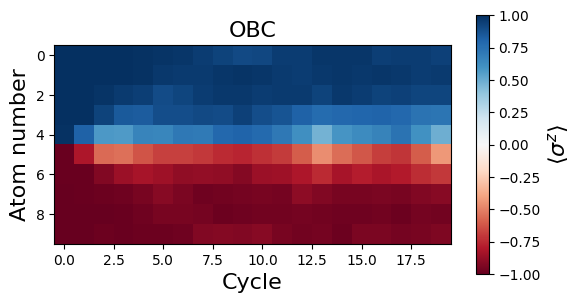
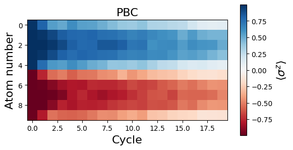
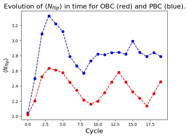
We see that the magnetization profiles look rather different for OBC and PBC. It seems that the initial DW melts in the case of PBC. In fact, the decrease of \(|\langle \sigma^z_j \rangle|\) for all sites is due to a delocalization of the DW along the circle. This delocalization can be more apparent when looking at correlations. More specifically, we see on the plot below that the number of spin flips between consecutive atoms along the circle, \(\langle N_{flip} \rangle=1/2\sum_j(1-\langle \sigma_j^z \sigma_{j+1}^z\rangle)\), remains quite low during the dynamics for both OBC (red) and PBC (blue), while it should tend to \(N_{at}/2=5\) for randomly distributed spins.

fig, ax = plt.subplots(1, 1)
plt.title(
    r"Evolution of $\langle N_{flip} \rangle$ in time for OBC (red) and PBC (blue).",
    fontsize=16,
)
ax.set_xlabel("Cycle", fontsize=16)
ax.set_ylabel(r"$\langle N_{flip} \rangle$", fontsize=14)
ax.plot(correl_pbc, "--o", color="blue")
ax.plot(correl_obc, "--o", color="red")

plt.show()

To investigate even more this delocalization effect, let’s consider a smaller region of only 3 spins prepared in \(|\uparrow \rangle\). The delocalization timescale will then be shorter, and we will see it more clearly happening in the system

N_cycles = 26
magnetizations_pbc = np.zeros((N_at, N_cycles), dtype=float)
samples_evol = []
masked_indices = [0, 1, 2]
for m in range(N_cycles):  # Runtime close to 4 min!
    seq = Sequence(reg, MockDevice)
    seq.set_magnetic_field(0.0, 0.0, 1.0)
    seq.declare_channel("MW", "mw_global")
    seq.config_slm_mask(masked_indices)
    seq.add(initial_pi_pulse, "MW")
    seq.add(X_pulse, "MW")
    Floquet_XX2Z_cycles(m, t_pulse)
    seq.add(mX_pulse, "MW")
    sim = QutipEmulator.from_sequence(seq)
    res = sim.run()
    samples = res.sample_final_state(N_samples)
    samples_evol.append(samples)
    correl = 0.0
    for key, value in samples.items():
        for j in range(N_at):
            magnetizations_pbc[j][m] += (
                (1 - 2 * float(key[j])) * value / N_samples
            )

fig, ax = plt.subplots(1, 1)
img = ax.imshow(magnetizations_pbc, cmap=plt.get_cmap("RdBu"))
ax.set_xlabel("Cycle", fontsize=16)
ax.set_ylabel("Atom number", fontsize=16)
cbar = fig.colorbar(img)
cbar.set_label(r"$\langle \sigma^z \rangle$", fontsize=16)
plt.show()

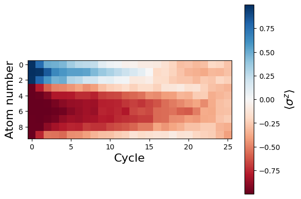
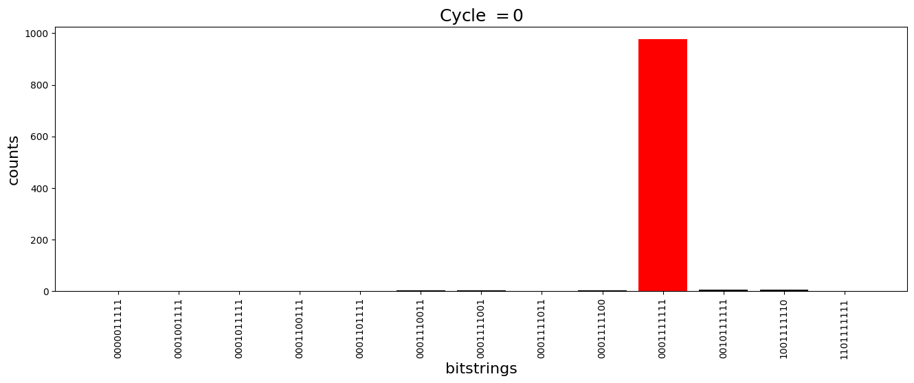
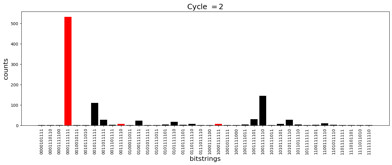
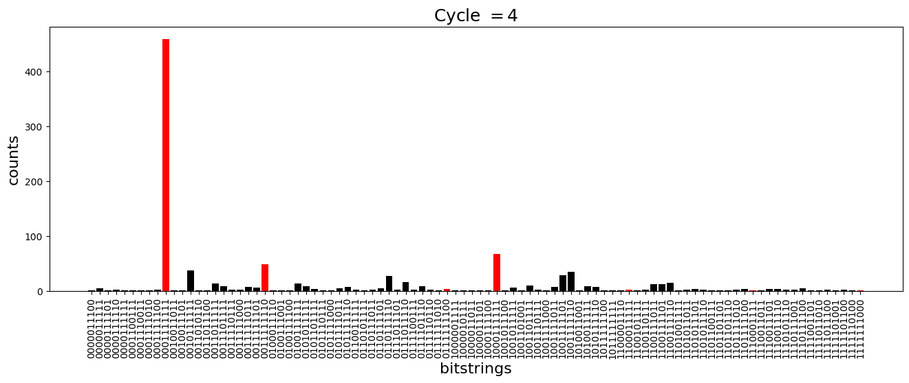
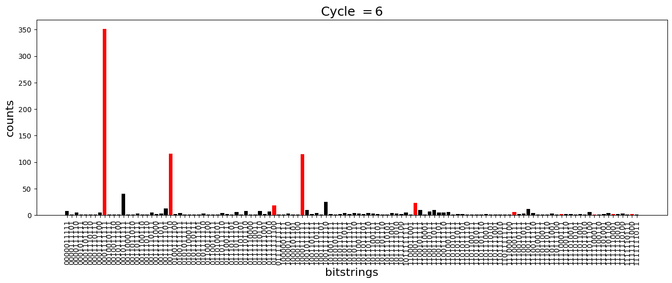
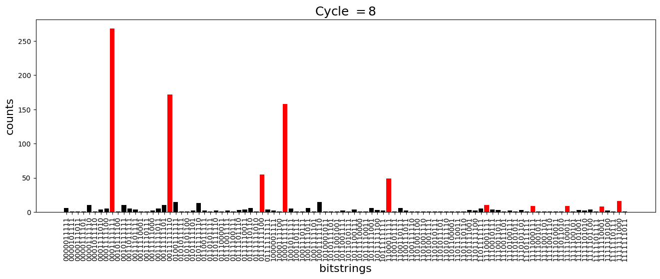
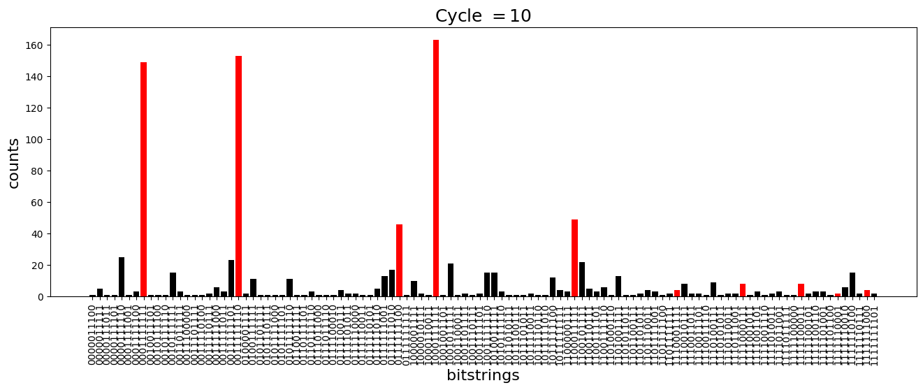
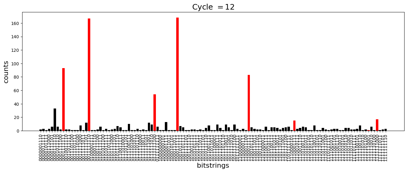
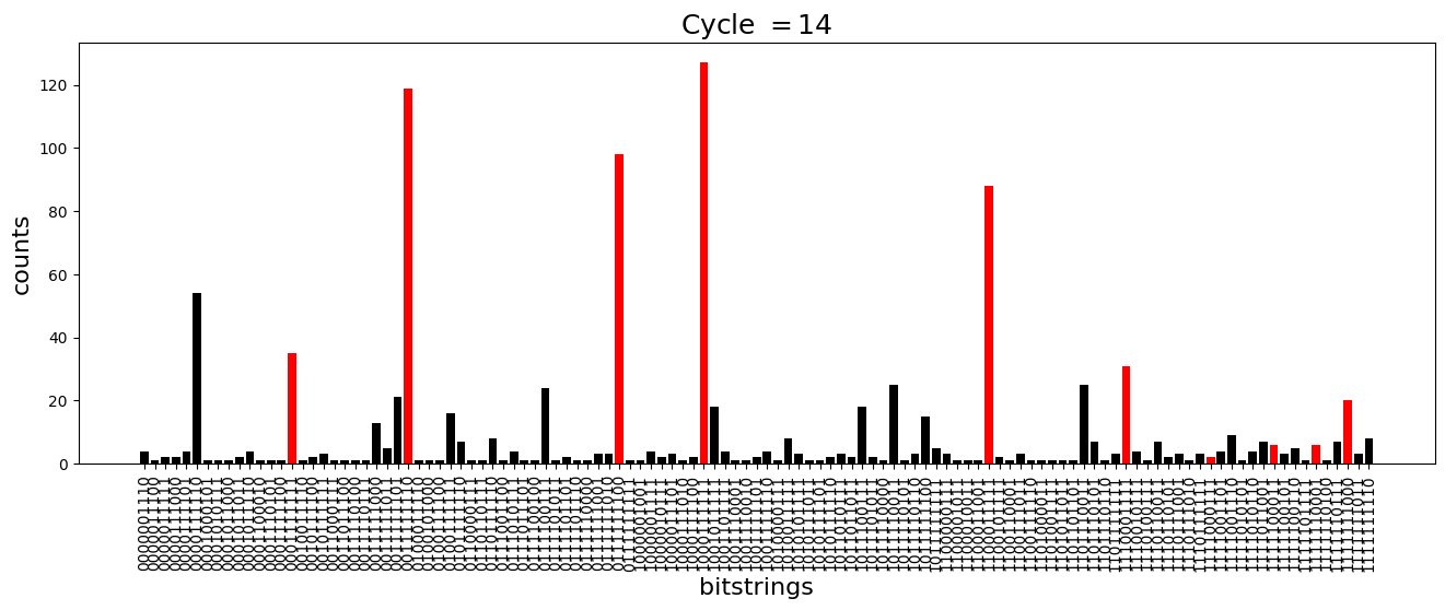
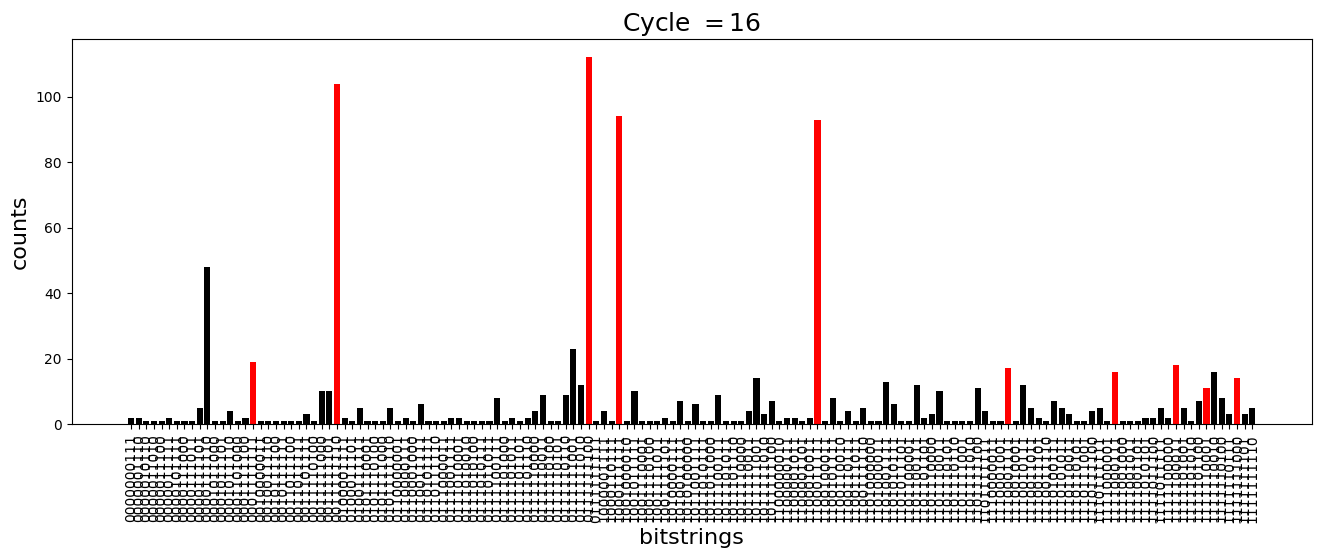
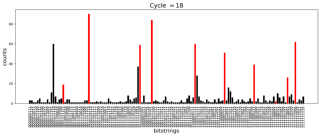
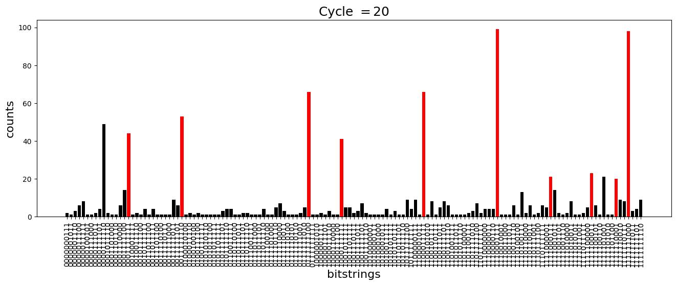
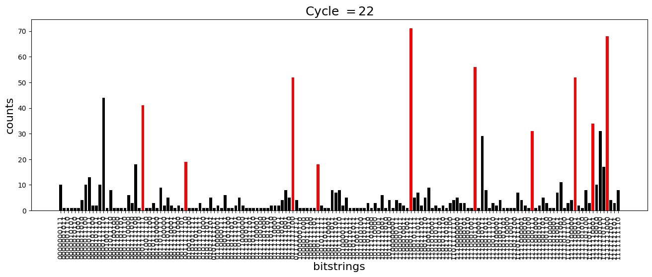
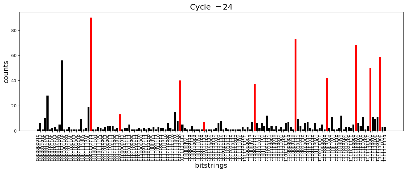
We see above that the magnetization profile tends to average. But if we look at the histogram of sampled states in time, we will remark that domain-wall configurations are dominant (in red in the histograms below). As time increases, the delocalization mechanism populates more and more domain-wall states distinct from the initial state.

dw_preserved = [
    "0001111111",
    "1000111111",
    "1100011111",
    "1110001111",
    "1111000111",
    "1111100011",
    "1111110001",
    "1111111000",
    "0111111100",
    "0011111110",
]

for n_cycle in [
    2 * k for k in range(int(N_cycles / 2))
]:  # Runtime close to 2 min !
    color_dict = {
        key: "red" if key in dw_preserved else "black"
        for key in samples_evol[n_cycle]
    }
    plt.figure(figsize=(16, 5))
    plt.title(r"Cycle $= {}$".format(n_cycle), fontsize=18)
    plt.bar(
        samples_evol[n_cycle].keys(),
        samples_evol[n_cycle].values(),
        color=color_dict.values(),
    )
    plt.xlabel("bitstrings", fontsize=16)
    plt.ylabel("counts", fontsize=16)
    plt.xticks(rotation=90)
    plt.show()